The Force Equilibrium Method

The force equilibrium method is a common method used to analyze the stability of slopes. It works for both circular and non-circular surfaces. It satisfies the force equilibrium equations for each slice, but it does not satisfy the moment equilibrium equations. There are several variations of the force equilibrium method, depending on the assumptions used for the side force inclination. In xslope, two variations of the force equilibrium method are supported: the Lowe and Karafiath method and the US Army Corps of Engineers method. Both methods use the same equations, but they differ in the side force assumptions. Because they satisfy force but not moment equilibrium, the computed factor of safety depends on the assumed side-force inclination and can be inaccurate — too high or too low — so these methods are best used for comparison, with a complete-equilibrium method such as Spencer preferred for design (see Conventions and Limitations below).

Forces Acting on the Slice

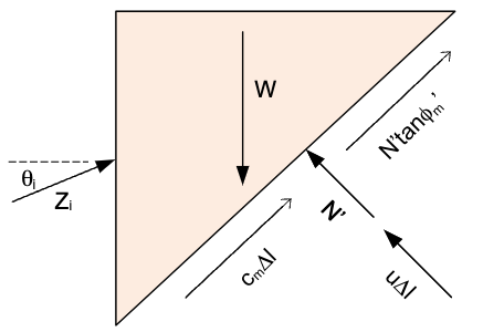
To formulate the force equilibrium equations, consider the following slice diagram:

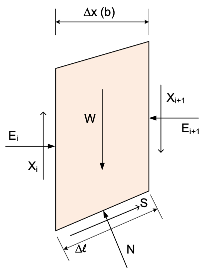
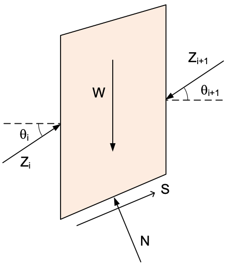
Note that the side forces are defined by the vertical (\(X_i\)) and horizontal (\(E_i\)) components of the force acting on the slice. The side forces can also be defined by the magnitude (\(Z_i\)) and the angle of inclination (\(\theta_i\)) of the force as follows:

The shear force (\(S\)) acting on the bottom of the slice is the mobilized shear strength of the soil, which is equal to:

\(S = \tau_m \Delta \ell\)

where \(\tau_m\) is the mobilized shear strength of the soil and \(\Delta \ell\) is the length of the slice. The mobilized shear strength is equal to:

\(\tau_m = \dfrac{c + (\sigma-u)\tan\phi}{F}\)

\(\tau_m = c_m + \sigma' \tan\phi_m\)

where:

• \(c\) = the cohesion of the soil
• \(c_m\) = the mobilized cohesion of the soil = \(c/F\)
• \(\sigma\) = the normal stress acting on the slice
• \(\sigma'\) = the effective normal stress acting on the slice = \(\sigma - u\)
• \(u\) = the pore water pressure acting on the slice
• \(\phi\) = the angle of internal friction of the soil
• \(\tan\phi_m\) = the mobilized friction of the soil = \(\tan\phi/F\)
• \(F\) = the factor of safety

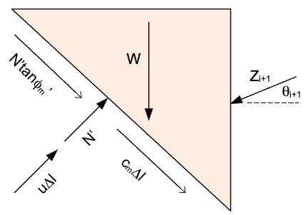
Inserting \(\tau_m\) into the equation for \(S\) gives:

\(S = \left[c_m + (\sigma') \tan\phi_m\right] \Delta \ell\)

\(S = c_m \Delta \ell + N' \tan\phi_m\)

where:

\(N'\) = the effective normal force acting on the slice = \(\sigma' \Delta \ell\)

\(N\) = the total normal force acting on the slice = \(N' + u \Delta \ell\)

Solving for Unknown Forces

To satisfy force equilibrium, we need to solve for the unknown forces acting on each slice. The ultimate goal is to solve for the factor of safety, F. However, the mobilized shear strength (\(c_m\) and \(\tan \phi_m\)) is a function of the factor of safety. Therefore, we first assume a value for the factor of safety and then solve the equilibrium equations for all slices. If the forces balance, we are done. If not, we adjust the factor of safety and repeat until balance is achieved. Also, the side force inclination (\(\theta\)) is required for all slice boundaries. There are a number of methods for establishing the side force inclination. These methods will be reviewed below. For now, we will assume we have a value for the side force inclinations.

So our next step is to use the force equilibrium equations to solve for the unknown forces acting on each slice. We do this by starting on the bottom slice (slice 1) and working our way up to the top slice (slice n). For the first slice, we have:

The unknowns in this case are the normal force (\(N'\)) and magnitude of the side force (\(Z_{i+1}\)). We do know the side force inclination (\(\theta_{i+1}\)). So we have two equations: \(\sum F_x = 0\) and \(\sum F_y = 0\) and two unknowns. After solving for the unknowns, we proceed to the next slice:

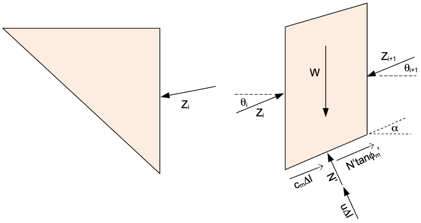
The side force on the left side (\(Z_{i-1}\)) is known from the previous slice. The side force on the right side (\(Z_ {i+1}\)) is unknown. The effective normal force (\(N'\)) is also unknown. So again, we have two equations and two unknowns.

We can continue this process until we reach the top slice:

At this point, there is no side force on the right side, so we have two equations and one unknown (\(N'\)), if both equilibrium equations are balanced (no residual forces), then the factor of safety is correct. If not, we need to adjust the factor of safety and repeat the process.

Matrix Solution for Unknown Forces

As shown in the previous section, we need to solve for two unknowns at each slice. For the general case, we can set up equations to solve for the unknowns as follows. First, we sum forces in the x-direction:

\(\sum F_x = 0 \Rightarrow \left[c_m \Delta \ell + N' \tan(\phi_m)\right] \cos(\alpha) - (N' + u \Delta \ell) \sin(\alpha) + Z_{i} \cos(\theta_i) - Z_{i+1} \cos(\theta_{i+1}) = 0\)

\(c_m \Delta \ell \cos(\alpha) + N' \tan(\phi_m) \cos(\alpha) - N' \sin(\alpha) - u \Delta \ell \sin(\alpha) - + Z_{i} cos (\theta_{i}) - Z_ {i+1} \cos(\theta_{i+1}) = 0\)

\(c_m \Delta \ell \cos(\alpha) + N' \left[\tan(\phi_m) \cos(\alpha) - \sin(\alpha)\right] - u \Delta \ell \sin(\alpha) + Z_{i} \cos (\theta_{i}) - Z_{i+1} \cos(\theta_{i+1}) = 0\)

Rearranging in terms of our two unknowns (\(N'\) and \(Z_{i+1}\)) gives:

\(N' \left[\tan(\phi_m) \cos(\alpha) - \sin(\alpha)\right] - Z_{i+1} \cos(\theta_{i+1}) = - c_m \Delta \ell \cos(\alpha) + u \Delta \ell \sin(\alpha) - Z_{i} \cos(\theta_i) \qquad (1)\)

Likewise, we can sum forces in the y-direction:

\(\sum F_y = 0 \Rightarrow \left[c_m \Delta \ell + N' \tan(\phi_m)\right] \sin(\alpha) + (N' + u \Delta \ell) \cos(\alpha) - W + Z_{i} \sin(\theta_{i}) - Z_{i+1} \sin(\theta_{i+1}) = 0\)

\(c_m \Delta \ell \sin(\alpha) + N' \tan(\phi_m) \sin(\alpha) + N' \cos(\alpha) + u \Delta \ell \cos(\alpha) - W + Z_{i} sin (\theta_{i}) - Z_{i+1} \sin(\theta_{i+1}) = 0\)

\(c_m \Delta \ell \sin(\alpha) + N' \left[\tan(\phi_m) \sin(\alpha) + \cos(\alpha)\right] + u \Delta \ell \cos(\alpha) - W + Z_{i} \sin (\theta_{i}) - Z_{i+1} \sin(\theta_{i+1}) = 0\)

Rearranging in terms of our two unknowns (\(N\) and \(Z_{i+1}\)) gives:

\(N' \left[\tan(\phi_m) \sin(\alpha) + \cos(\alpha)\right] - Z_{i+1} \sin(\theta_{i+1}) = -c_m \Delta \ell \sin(\alpha) - u\Delta \ell \cos(\alpha) + W - Z_{i} \sin(\theta_{i}) \qquad (2)\)

Now we can take equations (1) and (2) and rearrange them into a matrix form. We can write the two equations as:

\(Ax = b\)

where:

• \(A\) is a 2x2 matrix of coefficients
• \(x\) is a 2x1 vector of unknowns
• \(b\) is a 2x1 vector of constants

The matrix \(A\) is given by:

\(A = \begin{bmatrix}\tan(\phi_m) \cos(\alpha) - \sin(\alpha) & -\cos(\theta_{i+1})\\tan(\phi_m) \sin(\alpha) + \cos(\alpha) & -\sin(\theta_{i+1})\end{bmatrix} \qquad (3)\)

The vector \(x\) is given by:

\(x = \begin{bmatrix}N'\\Z_{i+1}\end{bmatrix} \qquad (4)\)

The vector \(b\) is given by:

\(b = \begin{bmatrix}- c_m \Delta \ell \cos(\alpha) + u \Delta \ell \sin(\alpha) - Z_{i} \cos(\theta_{i})\\-c_m \Delta \ell \sin(\alpha) - u\Delta \ell \cos(\alpha) + W - Z_{i} \sin(\theta_{i})\end{bmatrix} \qquad (5)\)

The matrix equation can then be solved for the two unknowns (\(N\) and \(Z_{i+1}\)) using the numpy linalg method. The solution is given by:

import numpy as np

N[i], Z[i + 1] = np.linalg.solve(A, b)

Complete Formulation

For a complete implementation of the Force Equilibrium method, we need to consider additional forces acting on the slice. The full set of forces are shown in the following figure:

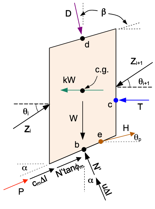
where:

\(D\) = distributed load resultant force
\(\beta\) = inclination of the distributed load (perpendicular to slope)
\(kW\) = seismic force for pseudo-static seismic analysis
\(c.g.\) = center of gravity of the slice
\(P\) = reinforcement force at point \(r\) on the base of the slice, at angle \(\psi\) from horizontal (\(\psi = \alpha\) for tangent/flexible reinforcement, the default; \(\psi\) = the line's own inclination for axial/rigid reinforcement)
\(T\) = tension crack water force
\(H\) = pile/pier force at point \(e\) on the failure surface
\(\theta_p\) = angle of pile force from horizontal (positive = counterclockwise/upward)
\(L\) = line load at point \(f\) on the top of the slice, at angle \(\delta\) from horizontal (default \(-90°\) = straight down)

⚠ TODO (figures): redraw the force diagram above in LibreOffice Draw — show \(P\) at a general angle \(\psi\) applied at point \(r\) (not tangent to the base), and add the line load \(L\) at angle \(\delta\) at point \(f\) on the top of the slice.

Each of these forces is described in detail in the Ordinary Method of Slices (OMS) section. The forces \(D\), \(kW\), \(P\), \(T\), \(H\), and \(L\) are included in the Force Equilibrium method as follows. Because the force-equilibrium method resolves each external force into global horizontal and vertical components, the generalization from tangent to axial reinforcement is immediate: \(P\cos(\alpha)\) and \(P\sin(\alpha)\) simply become \(P\cos(\psi)\) and \(P\sin(\psi)\). When Appl = Active (the default) \(P\) is not divided by \(F\); when Passive, the \(P\) terms are divided by \(F\) together with the soil strength (\(c_m\), \(\tan\phi_m\)).

Once again, we begin by summing forces in the x-direction, but now we include the additional forces. The pile force \(H\) at angle \(\theta_p\) has a horizontal component \(H \cos \theta_p\) that resists sliding (same direction as the reinforcement horizontal component \(P \cos \psi\)), and the line load contributes \(L \cos \delta\) (zero for a straight-down load):

\(\sum F_x = 0 \Rightarrow \left[c_m \Delta \ell + N' \tan (\phi_m)\right] \cos (\alpha) + P \cos (\psi) + H \cos \theta_p + L \cos \delta - (N' + u \Delta \ell) \sin (\alpha) + Z_{i} \cos (\theta_i) - Z_{i+1} \cos (\theta_{i+1}) + D \sin \beta - kW - T = 0\)

\(c_m \Delta \ell \cos (\alpha) + N' \tan (\phi_m) \cos (\alpha) + P \cos (\psi) + H \cos \theta_p + L \cos \delta - N' \sin (\alpha) - u \Delta \ell \sin (\alpha) + Z_{i} \cos (\theta_i) - Z_{i+1} \cos (\theta_{i+1}) + D \sin \beta - kW - T= 0\)

\(c_m \Delta \ell \cos (\alpha) + N' \left[\tan (\phi_m) \cos (\alpha) - \sin (\alpha)\right] + P \cos (\psi) + H \cos \theta_p + L \cos \delta - u \Delta \ell \sin (\alpha) + Z_{i} \cos (\theta_i) - Z_{i+1} \cos (\theta_{i+1}) + D \sin \beta -kW -T = 0\)

Rearranging in terms of our two unknowns (\(N'\) and \(Z_{i+1}\)) gives:

\(N' \left[\tan (\phi_m) \cos (\alpha) - \sin (\alpha)\right] - Z_{i+1} \cos (\theta_{i+1}) = - c_m \Delta \ell \cos (\alpha) - P \cos (\psi) - H \cos \theta_p - L \cos \delta + u \Delta \ell \sin (\alpha) - Z_{i} \cos (\theta_i) - D \sin \beta + kW + T \qquad (6)\)

It should be noted that the tension crack water force (\(T\)) only applies to right side of the top slice on a left-facing slope. For a right-facing slope, the tension crack water force is applied to the left side of the top slice and would act in the opposite direction. Therefore, the sign on \(T\) would be negative in that case.

Likewise, we can sum forces in the y-direction. The pile force has a vertical component \(H \sin \theta_p\) (upward for positive \(\theta_p\)), which acts in the same direction as the reinforcement vertical component \(P \sin \psi\); the line load contributes \(L \sin \delta\) (\(= -L\) for a straight-down load, i.e. it adds to the weight):

\(\sum F_y = 0 \Rightarrow \left[c_m \Delta \ell + N' \tan (\phi_m)\right] \sin (\alpha) + P \sin (\psi) + H \sin \theta_p + L \sin \delta + (N' + u \Delta \ell) \cos (\alpha) - W + Z_{i} \sin (\theta_{i}) - Z_{i+1} \sin (\theta_{i+1}) - D \cos \beta = 0\)

\(c_m \Delta \ell \sin (\alpha) + N' \tan (\phi_m) \sin (\alpha) + P \sin (\psi) + H \sin \theta_p + L \sin \delta + N' \cos (\alpha) + u \Delta \ell \cos (\alpha) - W + Z_{i} \sin (\theta_{i}) - Z_{i+1} \sin (\theta_{i+1}) - D \cos \beta = 0\)

\(c_m \Delta \ell \sin (\alpha) + N' \left[\tan (\phi_m) \sin (\alpha) + \cos (\alpha)\right] + P \sin (\psi) + H \sin \theta_p + L \sin \delta + u \Delta \ell \cos (\alpha) - W + Z_{i} \sin (\theta_{i}) - Z_{i+1} \sin (\theta_{i+1}) - D \cos \beta = 0\)

Rearranging in terms of our two unknowns (\(N'\) and \(Z_{i+1}\)) gives:

\(N' \left[\tan (\phi_m) \sin (\alpha) + \cos (\alpha)\right] - Z_{i+1} \sin (\theta_{i+1}) = -c_m \Delta \ell \sin (\alpha) - P \sin (\psi) - H \sin \theta_p - L \sin \delta - u\Delta \ell \cos (\alpha) + W - Z_{i} \sin (\theta_{i}) + D \cos \beta \qquad (7)\)

Now we can take equations (6) and (7) and rearrange them into a matrix form. We can write the two equations as:

\(Ax = b\)

The matrix \(A\) is given by:

\(A = \begin{bmatrix}\tan (\phi_m) \cos (\alpha) - \sin (\alpha) & -\cos (\theta_{i+1})\\\tan (\phi_m) \sin (\alpha) + \cos (\alpha) & -\sin (\theta_{i+1})\end{bmatrix} \qquad (8)\)

The vector \(x\) is given by:

\(x = \begin{bmatrix}N'\\Z_{i+1}\end{bmatrix} \qquad (9)\)

The vector \(b\) is given by:

\(b = \begin{bmatrix}- c_m \Delta \ell \cos (\alpha) - P \cos (\psi) - H \cos \theta_p - L \cos \delta + u \Delta \ell \sin (\alpha) - Z_{i} \cos (\theta_i) - D \sin \beta + kW + T\\-c_m \Delta \ell \sin (\alpha) - P \sin (\psi) - H \sin \theta_p - L \sin \delta - u\Delta \ell \cos (\alpha) + W - Z_{i} \sin (\theta_{i}) + D \cos \beta\end{bmatrix} \qquad (10)\)

Note that \(A\) and \(x\) are the same as before, but \(b\) has changed to include the additional forces. The matrix equation can then be solved for the two unknowns (\(N'\) and \(Z_{i+1}\)) using the numpy linalg method as described above.

Once again, care must be taken to ensure that the tension crack water force (\(T\)) is applied correctly based on the slope direction.

Side Force Inclination Assumptions

The side force inclination is a critical parameter in the force equilibrium method. Two solution methods are supported in xslope:

Lowe and Karafiath

The Lowe and Karafiath method assumes that the side force inclinations are equal to the average slope of ground surface and slip surface as defined by the top and bottom of the slice.

US Army Corps of Engineers

The US Army Corps of Engineers method assumes the side-force inclinations are parallel to the slope. The figure below (from EM 1110-2-1902) illustrates three such conventions; xslope implements the top and bottom ones:

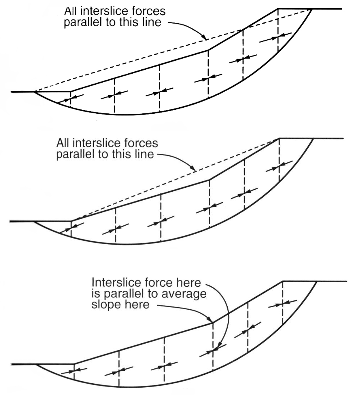
The convention is selected through the variant argument of corps:

• variant 1 (top panel) — a single constant inclination parallel to a line connecting the bottom of the failure surface to the top of the failure surface (the crest-to-toe chord). This matches the "Corps of Engineers #1" option in commercial packages.
• variant 2 (default) (bottom panel) — the inclination at each slice boundary is parallel to the ground surface at the top of that slice (the "Corps of Engineers #2" option).

The middle panel of the figure — all side forces parallel to the average embankment slope (a single straight line from the crest to the toe of the slope) — is a third Corps convention that xslope does not currently support. EM 1110-2-1902 (§C-4) notes that this average-embankment-slope assumption can yield unconservative (too-high) factors of safety relative to complete-equilibrium methods such as Spencer.

xslope defaults to variant 2. Because xslope can drive its own non-circular search, a single fixed inclination (variant 1) can return a spuriously low factor of safety on surfaces with steep segments — the search will seek out exactly those surfaces. The per-slice ground-parallel inclination (variant 2) is robust to this, which is why it is the default; variant 1 remains available to reproduce the "#1" results reported by other codes on a fixed surface.

Variant 2 is the default for robustness, not because it is conservative. The ground-parallel ("Corps #2") convention systematically produces the highest (least conservative) factor of safety among xslope's methods — typically a few percent to ~15% above Spencer. EM 1110-2-1902 cautions that methods which do not satisfy all conditions of equilibrium "may involve significant inaccuracies and should be used only under the restricted conditions described herein"; use a rigorous, complete-equilibrium method (Spencer) for design and report Corps for comparison.

Conventions and Limitations

The following apply to both the Lowe & Karafiath and Corps of Engineers methods, since they share xslope's force-equilibrium engine.

Inter-slice inclination sign convention. The force-equilibrium engine assembles slices from left to right with a fixed sliding sense. Both Corps conventions and Lowe & Karafiath therefore take the inter-slice inclination from the signed ground (or base) slope and negate it on right-facing slopes, so the computed factor of safety is the same for a slope and its mirror image. (A force-equilibrium factor of safety differing from Spencer's — in either direction — is expected given the side-force assumption, not a numerical error.)

Limitation — undrained (\(\phi = 0\)) surfaces with a dominant vertical load. Because the force-equilibrium methods satisfy only horizontal force equilibrium, they are unreliable on \(\phi = 0\) surfaces carrying a large vertical load (for example a submerged slope with ponded water modeled as a distributed load). In that configuration the horizontal force balance can be satisfied at a factor of safety several times larger than the true value — the method returns a genuine but grossly non-conservative root, not a numerical failure, so it is not caught by convergence checks. On a submerged \(\phi = 0\) test slope the Corps and Lowe & Karafiath factors of safety exceed the moment-method value (Ordinary = Bishop = Spencer) by a factor of three to five. Use a moment-satisfying method (Bishop, Spencer, Morgenstern-Price) for undrained or heavily surcharged slopes; the force-equilibrium methods are appropriate for drained, frictional materials.

References

• Lowe, J., and Karafiath, L. (1960). "Stability of earth dams upon drawdown." Proceedings of the First Pan-American Conference on Soil Mechanics and Foundation Engineering, Mexico City, Vol. 2, pp. 537–552.
• U.S. Army Corps of Engineers (2003). Slope Stability. Engineer Manual EM 1110-2-1902, Department of the Army, Washington, DC.
• Duncan, J. M., Wright, S. G., and Brandon, T. L. (2014). Soil Strength and Slope Stability, 2nd ed. John Wiley & Sons, Hoboken, NJ.