Sample Problems - Finite Element Method
Verification benchmarks (the Griffiths & Lane examples) are documented on the FEM/SSRM verification page.
The following examples illustrate how to use XSLOPE's finite element capabilities for slope stability analysis using the Shear Strength Reduction Method (SSRM). Each of the Excel input files below can be uploaded and used with the following Google Colab notebook which has been set up specifically for running FEM slope stability analyses:
![]()
The FEM implementation is described in the FEM Overview page.
1. Reinforced Slope with Geogrid Reinforcement
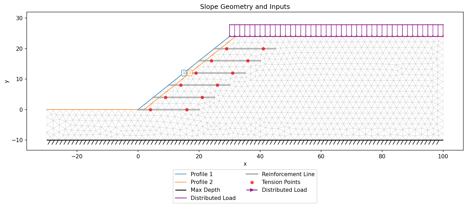
This problem features an engineered slope with six layers of geogrid reinforcement. It is the FEM counterpart of the LEM reinforced slope example described in the LEM Samples page (Problem 9). The slope geometry and soil properties are the same, with the addition of elastic modulus and Poisson's ratio for the FEM analysis:
| Property | Shell | Base |
|---|---|---|
| Cohesion, \(c\) (psf) | 300 | 0 |
| Friction angle, \(\phi\) (degrees) | 37 | 37 |
| Unit weight, \(\gamma\) (pcf) | 130 | 130 |
| Young's modulus, \(E\) (psf) | 1,000,000 | 1,000,000 |
| Poisson's ratio, \(\nu\) | 0.3 | 0.3 |
A 240 psf surcharge is applied along the slope crest from \(x = 30\) ft to \(x = 100\) ft.
Six reinforcement lines are defined with the following properties:
| Property | Value |
|---|---|
| \(T_{max}\) | 800 lb/ft |
| \(T_{res}\) | 600 lb/ft |
| \(L_{p1}\), \(L_{p2}\) | 4 ft |
| \(E\) | 800,000 psf |
| \(Area\) | 0.1 ft\(^2\)/ft |
| \(EA\) | 80,000 lb/ft |
Excel input file: xslope_reinforce_fem.xlsx
Inputs plotted with the XSLOPE plot_inputs() function:
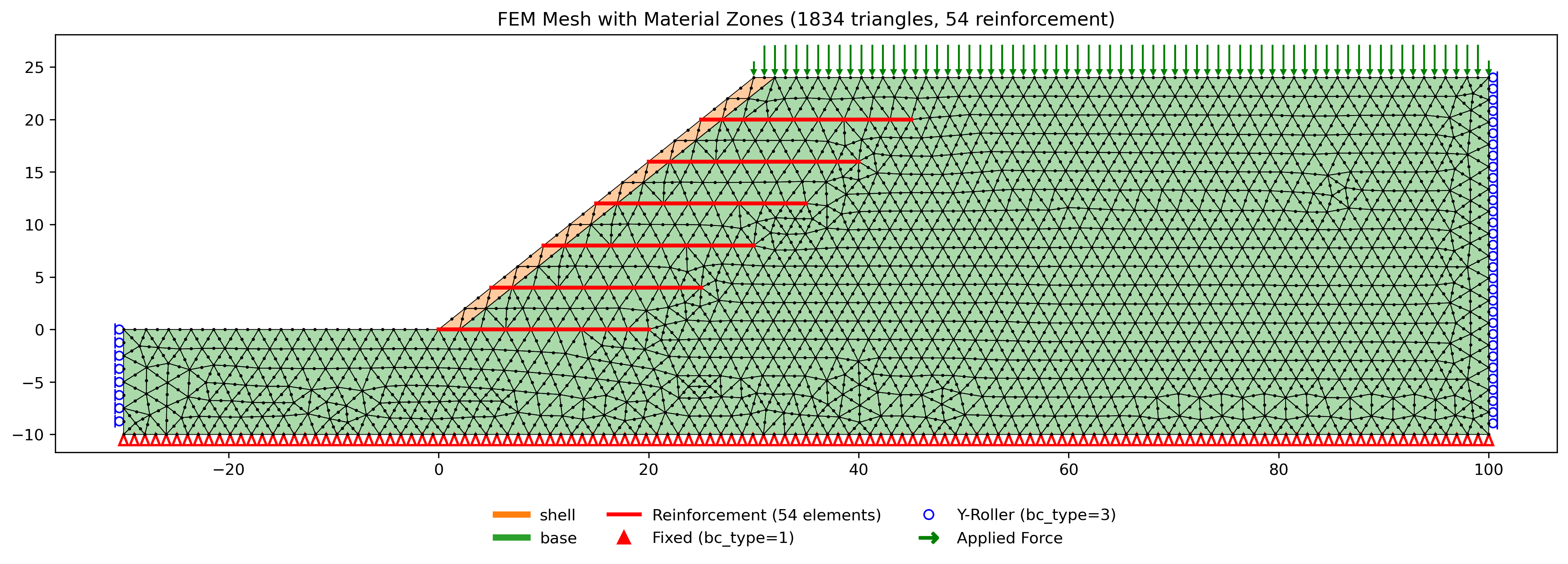
FEM mesh with boundary conditions and reinforcement elements (red lines):
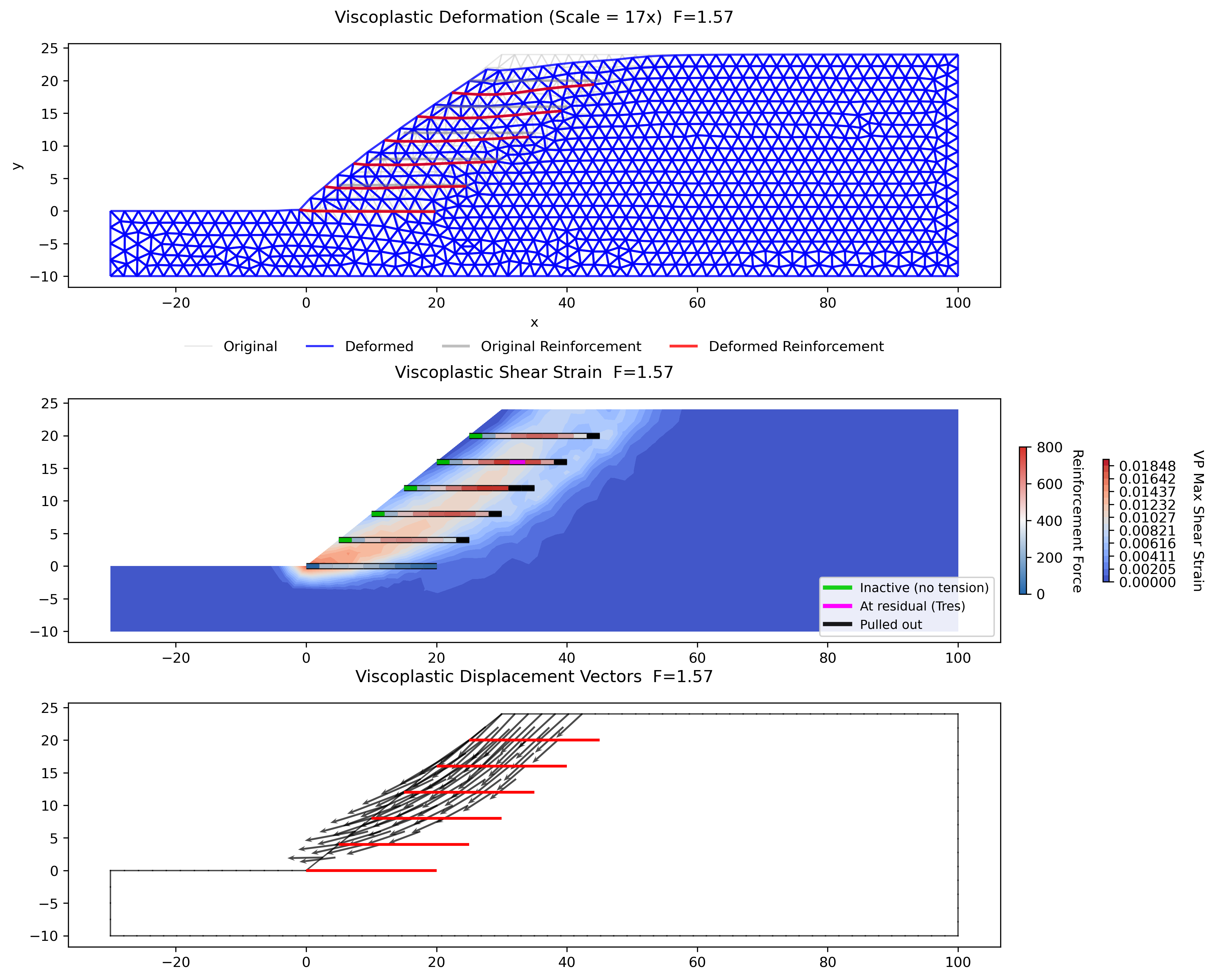
SSRM results. The computed factor of safety is FS = 1.49. The companion LEM analysis gives FS = 1.59 by Spencer's method (see LEM sample problem 9), and the FEM reads below it — as it should for this model, because this is a peak-residual run: \(T_{res}\) = 600 lb/ft is filled in, so reinforcement elements that yield shed down to their residual capacity, while the LEM has no strain compatibility and simply applies the full envelope value at each crossing (it ignores \(T_{res}\) entirely — see LEM Reinforcement).
That gap is the post-peak behavior, not a discrepancy between the methods. Blank out \(T_{res}\) and the same model runs elastic-perfectly-plastic at FS = 1.58, within 1% of the LEM — the two engines then agree closely, because they are finally assuming the same thing about the reinforcement.
The plots below show the solution at the computed factor of safety. The top plot shows the deformed mesh with original and deformed reinforcement positions. The middle plot shows the viscoplastic shear strain concentration with reinforcement elements colored by axial force (blue = low, red = high); green elements are inactive (no tension) and black elements at the ends have pulled out. The bottom plot shows the displacement vectors. The reinforcement summary table is shown below.
The print_reinforcement_summary() function reports the state of each line — how many
elements are carrying tension, how many sit inside a pullout ramp, how many have yielded,
and how many have dropped to the residual capacity — together with a status for the line:
| Status | Meaning |
|---|---|
| OK | All elements below capacity |
| NEAR CAPACITY | Peak force within 5% of \(T_{max}\) |
| PULLOUT | Elements near the ends have reached their embedment-limited capacity |
| YIELDED | Elements away from the ends are at \(T_{max}\) and holding it (perfectly plastic) |
| SOFTENED | Elements yielded and then dropped to \(T_{res}\) |
| INACTIVE | No elements carrying tension |
At the factor of safety the reinforcement is heavily mobilized: interior elements have reached \(T_{max}\) = 800 lb/ft and shed to \(T_{res}\) = 600 lb/ft, and elements inside the pullout ramps (\(L_p\) = 4 ft from each end) are limited by embedment rather than by material strength. This is the expected state at incipient failure — the slope fails when the soil's reduced strength and the reinforcement's residual capacity can no longer balance the driving forces together.
2. Slope Stabilized with Drilled Shaft Piles
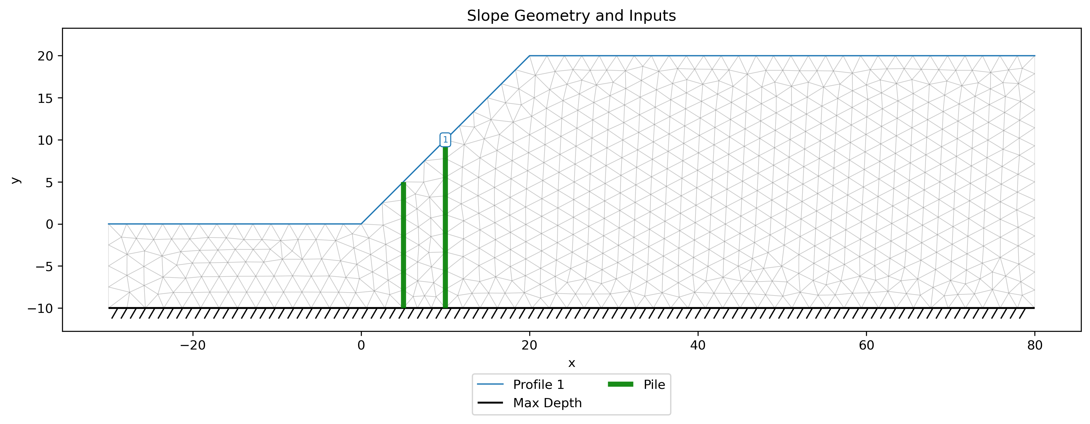
This problem features a 1:1 slope in a medium-stiff clay stabilized by two rows of drilled shafts.
Excel input file: xslope_piles_fem.xlsx
The soil properties are:
| Property | Value |
|---|---|
| Cohesion, \(c\) | 200 psf |
| Friction angle, \(\phi\) | 20 degrees |
| Unit weight, \(\gamma\) | 120 pcf |
| Young's modulus, \(E\) | 2,000,000 psf |
| Poisson's ratio, \(\nu\) | 0.3 |
Two rows of vertical drilled shafts are placed at \(x = 5\) ft and \(x = 10\) ft along the slope face, both extending from the ground surface to \(y = -10\) ft:
| Property | Value |
|---|---|
| Diameter, \(D\) | 2.0 ft |
| Spacing, \(S\) | 6.0 ft |
| Young's modulus, \(E_{\text{pile}}\) | 518,400,000 psf (concrete, \(f'_c\) = 4000 psi) |
| Moment of inertia, \(I\) | \(\pi D^4 / 64\) = 0.785 ft\(^4\) (auto-computed from \(D\)) |
| Cross-sectional area, \(A\) | \(\pi D^2 / 4\) = 3.14 ft\(^2\) (auto-computed from \(D\)) |
| Shear capacity, \(V_{\text{cap}}\) | 46,000 lb |
| Moment capacity, \(M_{\text{cap}}\) | 60,000 ft·lb |
| Fixity | free |
Each pile is modeled as a chain of 6-DOF Euler-Bernoulli beam elements with rotational DOFs at each node (see FEM Piles for the formulation). The pile stiffness (\(EI\) and \(EA\)) is scaled by \(1/S\) to convert from per-pile to per-unit-width quantities. Unlike the LEM approach where the user provides a single force \(H\), the FEM beam elements naturally develop resistance as the soil deforms around the pile. Bending moments are computed directly at each node, and structural capacity limits (\(V_{\text{cap}}\), \(M_{\text{cap}}\)) are enforced through the viscoplastic correction loop.
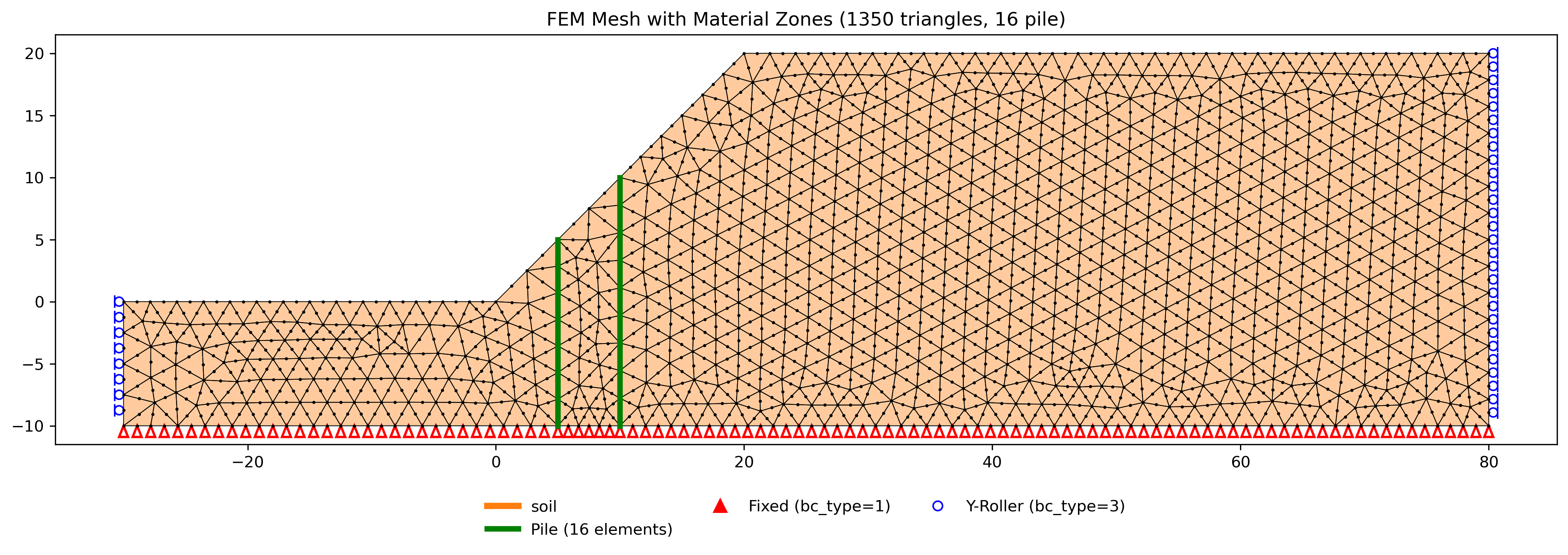
FEM mesh with boundary conditions. The piles are shown as green line elements along the pile axes:
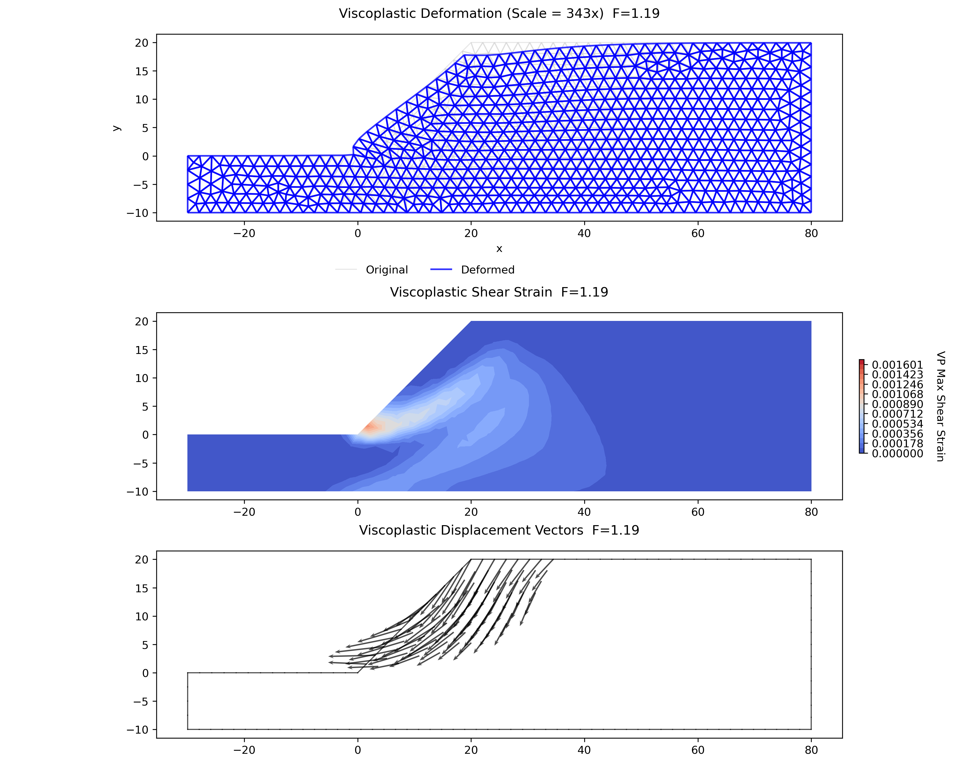
SSRM results without piles (FS = 1.18). The shear strain concentration shows a failure mechanism passing through the toe:
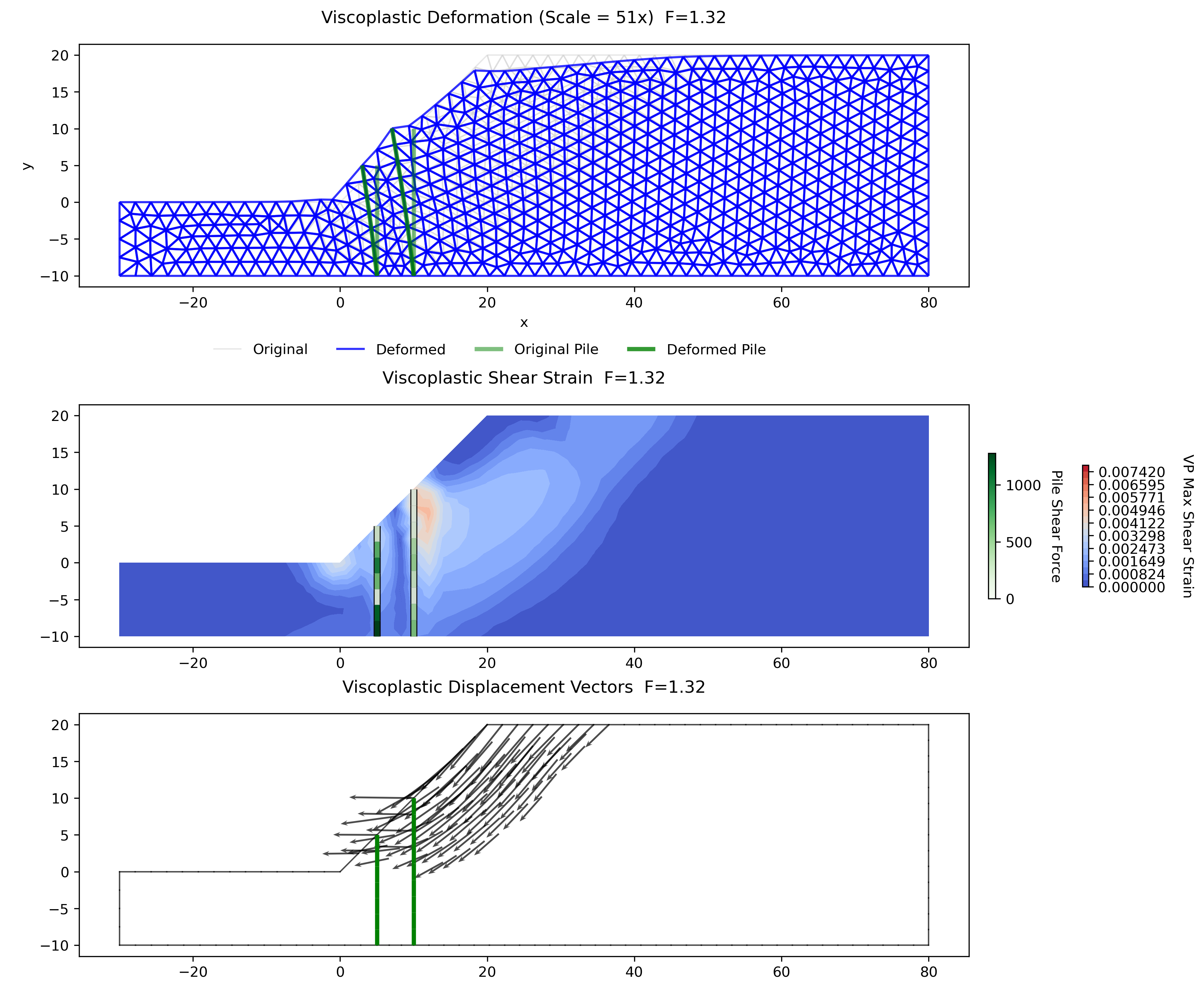
SSRM results with two rows of piles (FS = 1.36). The pile elements are colored by lateral (shear) force in the shear strain plot. The piles resist the sliding mass and the failure mechanism is modified by their presence:
Pile summary:
=== Pile Summary ===
Pile  Elems   Max |T|   Max |V|   Max |M|     V_cap     M_cap  Yielded  Status
--------------------------------------------------------------------------------
   1      7     482.1    2116.7    6352.4    7666.7   10000.0    0/7  OK
   2      9    1280.6    2323.6    7227.6    7666.7   10000.0    0/9  OK
--------------------------------------------------------------------------------
The two rows of piles increase the factor of safety from 1.18 to 1.36 — a 15% improvement. The maximum bending moment (7228 per unit width in Pile 2) reaches about 72% of the moment capacity (\(M_{\text{cap}}/S\) = 10,000), and the maximum shear about 30% of \(V_{\text{cap}}/S\), so the structural capacity does not govern for this problem. The soil's ability to transfer lateral load to the piles is the limiting factor, not the pile strength.
This is typical behavior for piles in relatively weak soil — the pile is much stiffer than the surrounding soil, and increasing the pile diameter or stiffness beyond a certain point produces diminishing returns. The 2D plane-strain model also does not capture the three-dimensional soil arching between piles that the Ito & Matsui theory accounts for in LEM, which can make the FEM result more conservative than the LEM result.
3. Non-Circular Failure Surface with Thin Weak Layer
This is the FEM counterpart of the LEM non-circular failure surface example described in the LEM Samples page (Problem 7). The problem features a thin weak clay layer in the foundation of a slope, which controls the failure mechanism. This problem was also featured in the user manual for the UTEXASED slope stability analysis software developed by Stephen G. Wright at the University of Texas at Austin.
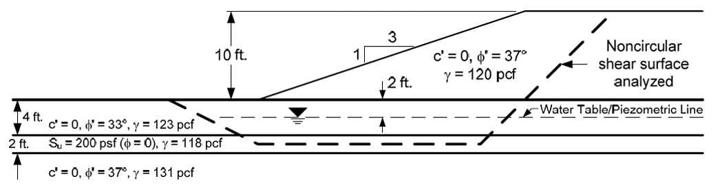
The slope geometry and strength properties are the same as the LEM problem. Young's modulus (\(E\)) and Poisson's ratio (\(\nu\)) are estimated from typical correlations for each soil type:
| Soil | \(c'\) (psf) | \(\phi'\) (deg) | \(\gamma\) (pcf) | \(E\) (psf) | \(\nu\) |
|---|---|---|---|---|---|
| Sand Fill | 0 | 37 | 120 | 1,000,000 | 0.30 |
| Sand | 0 | 33 | 123 | 700,000 | 0.30 |
| Soft Clay (\(S_u\) = 200) | 0 (\(\phi = 0\)) | 0 | 118 | 60,000 | 0.40 |
| Dense Sand | 0 | 37 | 131 | 1,500,000 | 0.28 |
The soft clay is modeled as an undrained material (\(\phi = 0\)) with \(E/S_u \approx 300\). A Poisson's ratio of 0.40 is used rather than the theoretical undrained value of 0.5 to avoid numerical issues with near-incompressibility.
Excel input file: xslope_noncircular_fem.xlsx
Inputs plotted with the XSLOPE plot_inputs() function:
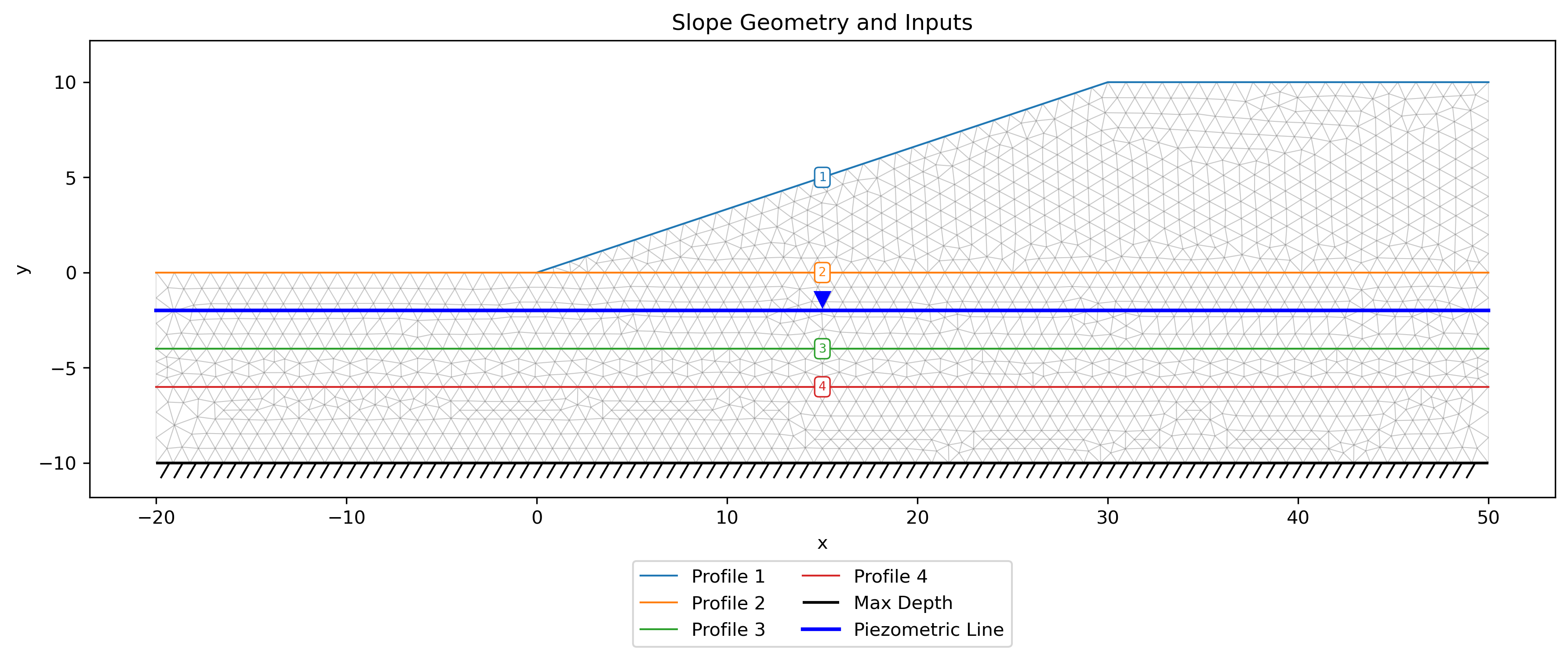
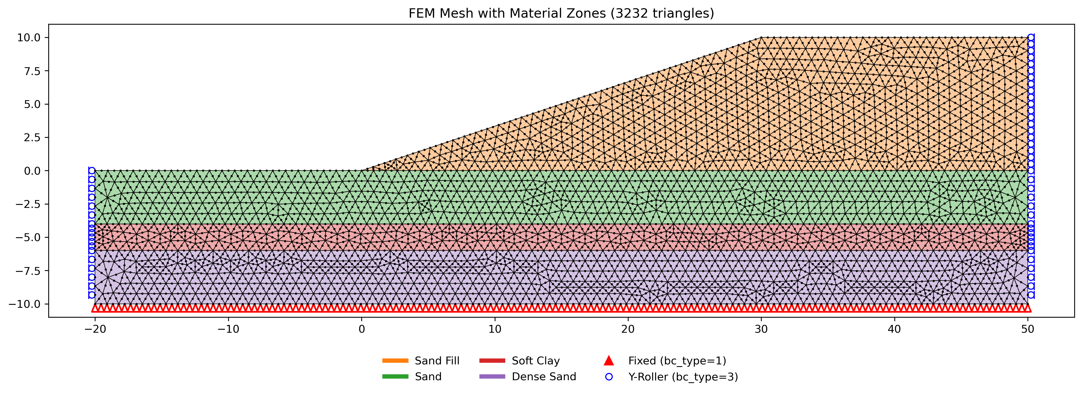
FEM mesh with boundary conditions and material zones. Mesh resolution matters for this problem: the soft clay layer is only 2 ft thick, and the mesh must place at least two elements through its thickness to resolve the shear band that controls the failure mechanism — a target element size of 1.0 ft (or finer) is required. A coarser mesh stiffens the thin layer artificially and distorts the strain field within it:
SSRM results. The computed factor of safety is FS = 1.59. The plots show the solution at the computed factor of safety. The middle plot shows the viscoplastic shear strain concentration, which clearly reveals the non-circular failure mechanism passing through the thin weak clay layer — matching the expected behavior without any prior assumption about the failure surface shape. The bottom plot shows the displacement vectors, confirming lateral sliding of the slope mass along the clay layer.
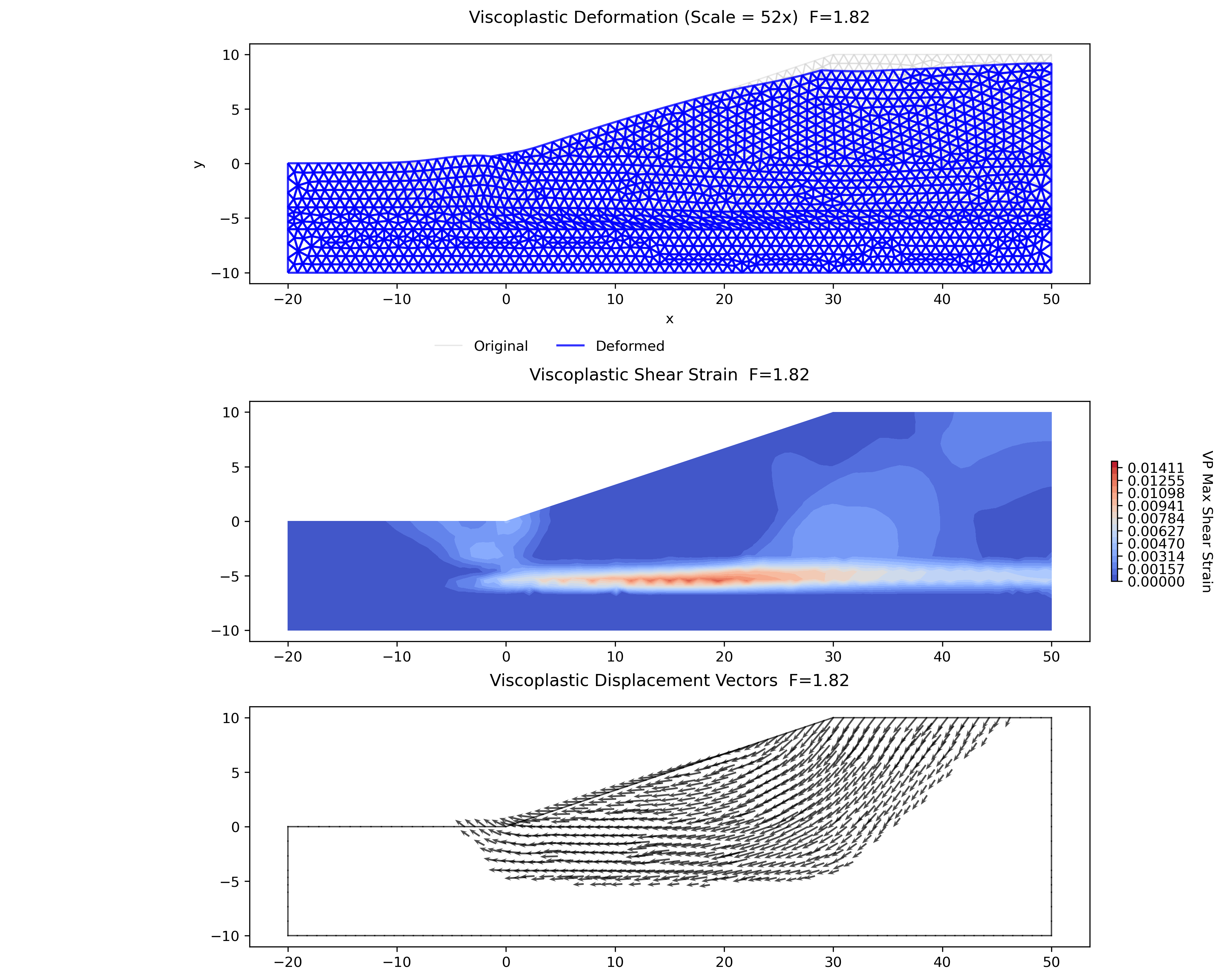
The FEM result of FS = 1.59 is about 9% below the LEM result of FS = 1.74 obtained using Spencer's method — both analyses use the same piezometric surface in the foundation sand. Differences of this order between SSRM and LEM are typical: the FEM develops the failure mechanism freely through the global stress field, while the LEM evaluates rigid-block equilibrium on a prescribed surface, and the two methods answer subtly different questions. The FS shows a mild residual mesh sensitivity characteristic of thin-shear-band localization (1.64 / 1.59 / 1.55 at target sizes 2.0 / 1.0 / 0.75): the finer the mesh, the more sharply the band through the 2-ft layer is resolved.
4. Reliability Analysis: Two-Layer c–φ Slope
This example demonstrates a finite-element reliability analysis — the same Taylor Series Probability Method as the LEM reliability analysis, but with each factor of safety computed by SSRM. See Reliability Analysis (FEM) for the method.
Excel input file: xslope_simple_mult_layers_fem.xlsx
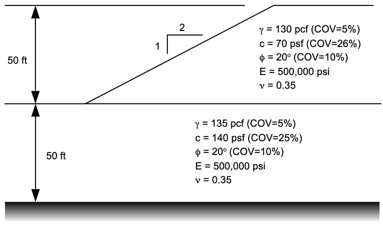
It reuses the geometry of the LEM Simple Slope with Multiple Layers example — an embankment over a foundation layer — with the elastic properties (\(E\), \(\nu\)) added for the finite-element solve and the strength retuned to a marginally stable c–φ slope so the reliability is interesting rather than near-certain:
| Material | \(c\) | \(\phi\) | \(\gamma\) | \(E\) | \(\nu\) | \(\sigma_c\) (COV) | \(\sigma_\phi\) (COV) | \(\sigma_\gamma\) (COV) |
|---|---|---|---|---|---|---|---|---|
| Embankment | 70 | 20° | 130 | 500,000 | 0.35 | 18 (26%) | 2 (10%) | 6.5 (5%) |
| Foundation | 140 | 20° | 135 | 500,000 | 0.35 | 35 (25%) | 2 (10%) | 6.75 (5%) |
Running the analysis (reliability_fem, or Studio → Run FEM → Reliability)
on a tri6 mesh (50 divisions across the width, target_size ≈ 2.4, ~2080 nodes)
gives:
| \(F_{MLV}\) | \(\sigma_F\) | \(COV_F\) | \(\beta_{LN}\) | Reliability \(R\) | \(P_f\) |
|---|---|---|---|---|---|
| 1.143 | 0.122 | 0.107 | 1.196 | 88.4% | 11.6% |
The most-likely factor of safety is only 1.14, so despite the moderate parameter scatter the probability of failure is a non-trivial ≈11.6% — a reminder that a factor of safety comfortably above 1.0 does not by itself imply a low failure probability.
The per-parameter ΔF table also shows which uncertainties matter:
| Parameter | MLV | σ | \(F^+\) | \(F^-\) | ΔF |
|---|---|---|---|---|---|
| Embankment \(\phi\) | 20 | 2 | 1.235 | 1.052 | 0.182 |
| Embankment \(c\) | 70 | 18 | 1.220 | 1.059 | 0.160 |
| Embankment \(\gamma\) | 130 | 6.5 | 1.127 | 1.159 | 0.031 |
| Foundation \(\phi\) | 20 | 2 | 1.143 | 1.143 | 0.000 |
| Foundation \(c\) | 140 | 35 | 1.143 | 1.143 | 0.000 |
| Foundation \(\gamma\) | 135 | 6.75 | 1.143 | 1.143 | 0.000 |
The foundation's properties have ΔF = 0: the critical failure mechanism is confined to the weaker embankment and never reaches the stronger foundation, so its strength and its uncertainty have no effect on the factor of safety. The embankment's friction angle and cohesion dominate the reliability. This is a useful by-product of the Taylor Series method — it exposes each parameter's contribution directly.
The result depends on the mesh — but not on the bracket
These numbers are for the tri6 mesh above. A finer or different-element mesh
gives a slightly different factor of safety and hence reliability — the FEM
factor of safety converges downward toward the LEM value as the mesh refines
(this slope: quad8 at target_size 2 → FS ≈ 1.25, matching LEM's 1.244). For a
fixed mesh, though, the reliability is fully reproducible: reliability_fem
runs each SSRM on a fixed global grid, so the result is identical to every
decimal regardless of the F_min/F_max bracket — see
Numerical precision.
An homage to Griffiths & Lane (1999). XSLOPE's finite-element slope-stability solver was built on the methodology of Griffiths & Lane (1999), "Slope stability analysis by finite elements" (Géotechnique 49(3), 387–403) — a plane-strain elasto-plastic (Mohr–Coulomb) formulation solved by viscoplastic strength reduction, with the factor of safety located by the non-convergence criterion. In tribute to that lineage, the verification set now reproduces all six of the paper's worked examples:
- Example 1 — homogeneous slope
- Example 2 — foundation layer, the false base circle
- Example 3 — undrained clay with a thin weak layer — figure-read Fig. 7 sweep and the two-mechanism showcase
- Example 4 — undrained clay over a weak foundation — the base→toe mechanism flip
- Example 5 — "slow" drawdown sweep — a pore-pressure and reservoir-load showcase
- Example 6 — two-sided earth dam
Each is documented in full — geometry, mesh, factor of safety, and the locked regression tags — on the FE Slope Stability (SSRM) verification page, which also carries the two-tier Verification overview.