DXF Import/Export

XSLOPE exchanges geometry with CAD software through the DXF format, using the xslope.cad module. There are three things you can do:

• Export a model to DXF — write a complete model out to a layered DXF for documentation, sharing, or editing in CAD (export_dxf).
• Import polygons from a DXF — read material-zone polygons from a DXF and write them to the polygons sheet of an input template (import_dxf).
• Save a plot to DXF — save any XSLOPE plot (inputs, solution, search, seepage, FEM) directly to a layered DXF, the analog of saving a PNG (save_dxf=True).

The common thread across all three is layers: when XSLOPE writes a DXF it places each feature or plotted artifact on its own named layer, and when it reads a DXF it uses layer names to identify materials. Layer names are uppercased, with spaces and DXF-illegal characters (< > / \ " : ; ? * | = plus the backtick) replaced by underscores — so a material named "Silty Clay" becomes layer SILTY_CLAY.

---

Exporting a model to DXF

The export_dxf function in the xslope.cad module writes everything present in the loaded model to a layered DXF:

from xslope.fileio import load_slope_data
from xslope.cad import export_dxf

slope_data = load_slope_data("my_slope.xlsx")
export_dxf(slope_data, "my_slope.dxf")          # DXF version R2010 by default

Each feature in the model is written to a named layer:

Model feature	DXF entity	Layer
Material zones	closed LWPOLYLINE	one per material, named after it (e.g. CLAY_CORE)
Profile lines	open LWPOLYLINE	PROFILE_<material>
Failure surface	LWPOLYLINE	FAILURE_SURFACE
Search circles	CIRCLE + POINT	SEARCH_CIRCLES
Reinforcement lines	LINE	REINFORCEMENT
Distributed loads	LWPOLYLINE	DLOADS
Piezometric / water table	LWPOLYLINE	PIEZO

Material-zone layers are named after the material itself. Every other layer above (the PROFILE_ prefix and the fixed feature names) is a reserved name — these are the layers that import recognizes and skips, since import reads only material zones (see below).

The result opens directly in any CAD program, with each feature on a layer you can show, hide, or restyle.

A real example, exported from the Earth Dam sample: xslope_earth_dam_up.dxf — material zones (SHELL, CORE, CLAY, SAND), the profile lines, the piezometric line, the distributed load, and the search circles, each on its own layer.

Excel input file: xslope_earth_dam_up.xlsx

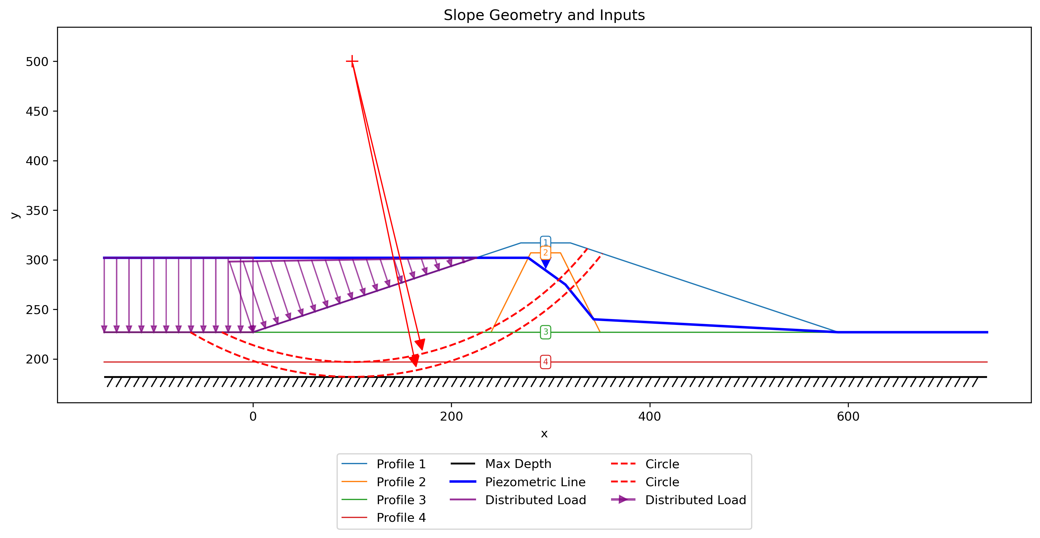
Inputs plotted with the XSLOPE plot_inputs() function:

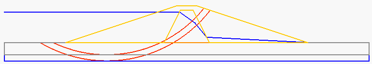
Exported DXF file: xslope_earth_dam_up.dxf

Exported DXF file opened in CAD:

---

Importing polygons from a DXF

Import reads geometry in the other direction: a DXF drawing of a cross-section becomes the polygons sheet of an input template.

Step 1 — Organize the CAD drawing

Draw each material zone as a closed polyline on a layer named after the material. All polylines on a layer are assigned to the same material. The importer is tolerant of common real-world variations:

• both lightweight LWPOLYLINE and heavyweight POLYLINE entities,
• arc segments (polyline bulges) — tessellated to straight segments,
• unclosed polylines — closed automatically (with a warning),
• a zone drawn as loose LINE segments — stitched into a ring by shared endpoints.

Step 2 — Review the extracted zones

Before importing, print a summary to confirm the extraction — that the right zones were found, the geometry looks correct, and nothing is missing or duplicated:

from xslope.cad import summarize_dxf

summarize_dxf("my_slope.dxf")

Poly ID │ Layer Name         │ Vertices │       Area
────────┼────────────────────┼──────────┼───────────
      1 │ EMBANKMENT         │        4 │    2000.00
      2 │ FOUNDATION         │        4 │    4250.00

Unique material layers (2): EMBANKMENT, FOUNDATION

Step 3 — Import into a template

import_dxf copies an input template, writes the extracted polygons to the polygons sheet, and seeds the mat sheet with the layer names as material names:

from xslope.cad import import_dxf

result = import_dxf(
    "my_slope.dxf",                          # source DXF
    "docs/inputs/input_template.xlsx",       # template to copy
    "my_slope.xlsx",                         # output input file
)
print(result["layer_to_mat"])   # {'EMBANKMENT': 1, 'FOUNDATION': 2}
print(result["warnings"])       # e.g. ["open polyline on layer 'SAND' auto-closed"]

By default each unique layer (in first-appearance order) is assigned material IDs 1, 2, 3, …. To control the mapping, pass material_map:

import_dxf(
    "my_slope.dxf", "docs/inputs/input_template.xlsx", "my_slope.xlsx",
    material_map={"EMBANKMENT": 1, "FOUNDATION": 2},
)

For finer control, the underlying reader is available directly:

from xslope.cad import dxf_to_polygons

polygons, warnings = dxf_to_polygons("my_slope.dxf")   # optional: layers=[...]
# polygons -> [{'coords': [(x, y), ...], 'layer': 'EMBANKMENT'}, ...]

Step 4 — Fill in material properties

Import seeds only the material names. Open the generated my_slope.xlsx, go to the mat sheet, and fill in the strength and other properties for each material. The file is not analysis-ready until the material properties are provided.

---

Saving a plot to DXF

Any XSLOPE geometry plot can be saved directly to a layered DXF with a save_dxf=True argument — the exact analog of the existing save_png option. Unlike export_dxf (which writes the input model), this captures what the plot shows — slices, stress diagrams, the critical surface, contours, the mesh — so it works for solution, search, seepage, and FEM plots:

from xslope.plot import plot_inputs, plot_solution, plot_circular_search_results

plot_inputs(slope_data, save_dxf=True)
plot_solution(slope_data, slice_df, surface, results, save_dxf=True)
plot_circular_search_results(slope_data, fs_cache, save_dxf=True)

from xslope.plot_seep import plot_seep_solution
from xslope.plot_fem import plot_fem_results

plot_seep_solution(seep_data, solution, save_dxf=True)   # flow net + contours
plot_fem_results(fem_data, solution, plot_type=['deformation', 'shear_strain'],
                 save_dxf=True)                           # one DXF per panel

The DXF is named like the PNG the plot would save (e.g. plot_spencer_fs_=_1.242.dxf). FEM result figures are multi-panel, so they write one DXF per plot type (fem_results_deformation.dxf, fem_results_shear_strain.dxf, …).

Each plotted artifact lands on its own layer:

Plot	DXF layers
Inputs / solution	one layer per material zone, MAX_DEPTH, SLICES, FAILURE_SURFACE, EFF_NORMAL_STRESS, PORE_PRESSURE, LINE_OF_THRUST, PIEZO, DLOADS, TENSION_CRACK, CIRCLES
Search results	CRITICAL_SURFACE, TESTED_SURFACES, CIRCLE_CENTERS, SEARCH_PATH
Seepage	HEAD_CONTOURS, FLOWLINES, PHREATIC, CONTOUR_FILL, ZONE_FILL, MESH, MESH_BOUNDARY, MESH_NODES, SEEP_FIXED_HEAD, SEEP_EXIT_FACE
FEM	MESH, MESH_FILL, <quantity>_CONTOURS (e.g. VP_MAX_SHEAR_STRAIN_CONTOURS), STRESS_CONTOURS, REINFORCEMENT, PILES

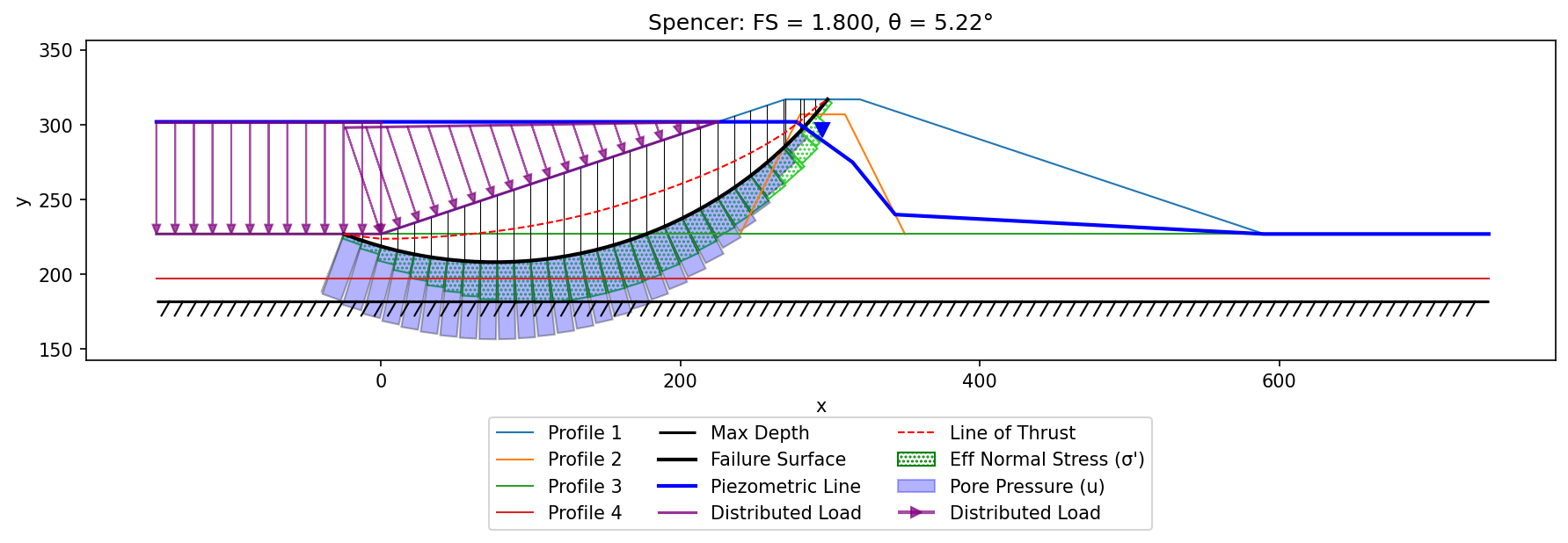
PNG generated from the plot_solution function:

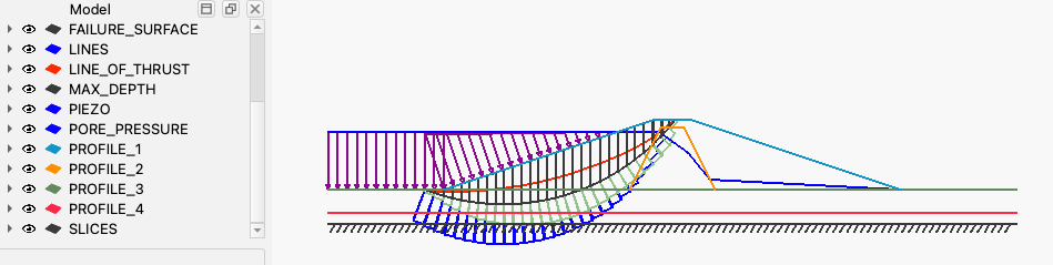
DXF file generated from the same plot using the save_dxf option:

---

Notes and limitations

• Import is polygons-only. Other features (piezo, loads, circles) are entered in the template; export and plot-saving write them, but import ignores their reserved layers.
• Material properties are not in the DXF. Import seeds names only; properties are filled in on the mat sheet afterward.
• Round-trip. Exporting a model and re-importing it reproduces the material-zone geometry exactly (feature layers are written by export but ignored on import).
• Format. DXF only for now. DWG requires Autodesk libraries or the ODA File Converter and may be added based on demand.