Rocscience Slide2 Groundwater Corpus
This page tracks the Slide2 Groundwater Verification Manual
(Rocscience, 2022; 21 problems) the same way the Slide2 slope-stability corpus
tracks its manual: every problem gets a row, built problems get an XSLOPE input file
(docs/verification/files/rocscience_gw/), a results section, and regression test tags. Unlike the LEM
corpus, the seepage tags mesh and solve live on every run — the committed artifact is the
input file alone.
Full bibliographic details for the author-year citations on this page are on the shared References page.
The manual verifies Slide2's finite-element groundwater engine against closed-form solutions (Polubarinova-Kochina, Vedernikov, Terzaghi consolidation) and published numerical benchmarks. It is the seepage analog of the slope-stability manual, and the natural verification target for XSLOPE's own FE seepage solver — which the LEM corpus already exercises end-to-end on VP71, VP72, VP76, VP77 and VP102, but only as a pore-pressure source, not against seepage-specific quantities (flow rates, free-surface positions, pressure profiles).
Problems 1–13 are steady-state and analyzable with the current solver. Problems 15–21 are transient (and 15–16 are consolidation), which XSLOPE's steady-state solver does not support.
One capability is deliberately out of scope, so the rows that depend on it are blocked by design rather than pending work:
- Transient seepage. XSLOPE's seepage analysis exists to supply pore pressures to a stability analysis, and a transient head field does not change a factor of safety on its own — capturing rainfall-induced failure would additionally require an unsaturated shear-strength model (such as Fredlund's \(\phi^b\)), without which suction is neglected in the stability calculation regardless of how the water table moves. Rapid drawdown, the other classic transient case, is already covered by the staged Duncan & Wright procedure that is standard of practice. Problems 16–21 are blocked on this.
Problems 1, 7, 8 and 14 apply a uniform infiltration rate to the ground surface, which has no
fixed-head equivalent. These require a
specified-flux (Neumann) boundary condition,
which the solver now supports. Three of them — 1 (Dupuit recharge mound), 7 (Rulon &
Freeze layered slope) and 8 (ditch-drained aquifer) — are built on that boundary. The fourth,
14, turned out to be blocked for a different reason: its published quantity is the Gardner
(1958) capillary profile, which is derived for the exponential conductivity law
\(k = k_s\,e^{\alpha\psi}\) — a law XSLOPE does not implement (its gard option is the power form
\(k_r = 1/(1 + a\,\psi^n)\) that SEEP/W and Slide carry, a different function). With no exponential
law and no tabulated Slide value to compare against (the manual prints only Fig. 14.3/14.4 charts),
there is nothing to lock beyond a one-dimensional through-flux the flux cross-check already verifies
to machine precision, so GW14 is blocked rather than tuned to a substitute curve.
Status
| # | Problem | Status | Notes |
|---|---|---|---|
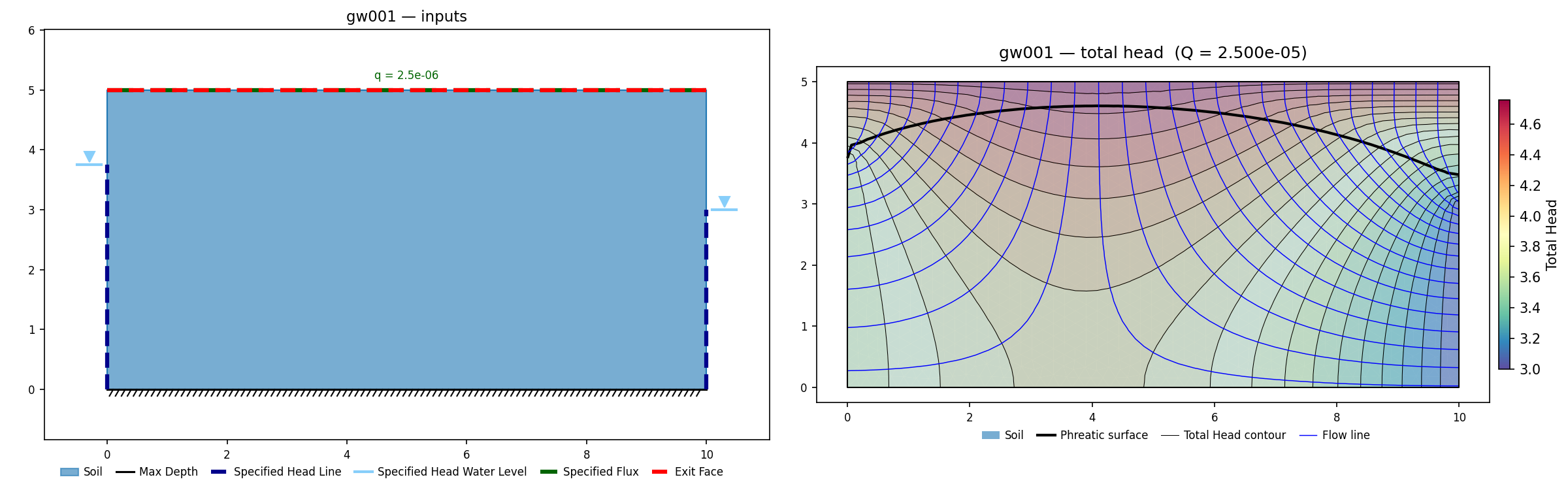
| 1 | Shallow unconfined flow with rainfall | built | gw001.xlsx. Dupuit recharge mound between two rivers, P = 2.5×10⁻⁶ m/s applied as a specified flux. The free-surface crest reads x_a ≈ 4.1, h_max ≈ 4.61 vs Slide 4.06 / 4.49 and Haar's closed form 3.98 / 4.25 — a touch above Slide, the same free-surface-family bias the SEEP2D cross-check documents. Q = P·L = 2.5×10⁻⁵ locked. |
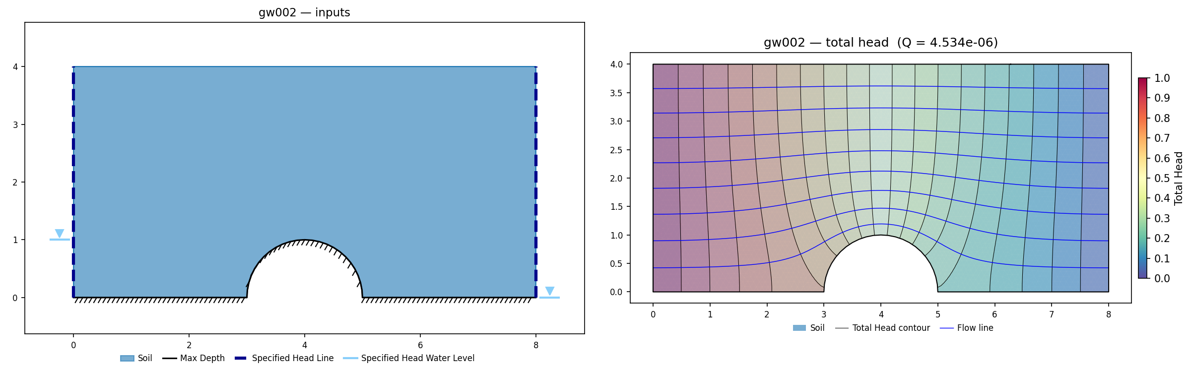
| 2 | Flow around cylinder | built | gw002.xlsx. Confined potential flow: solved heads match Slide within 0.0013 m at every printed point and the closed form within its own idealization error. |
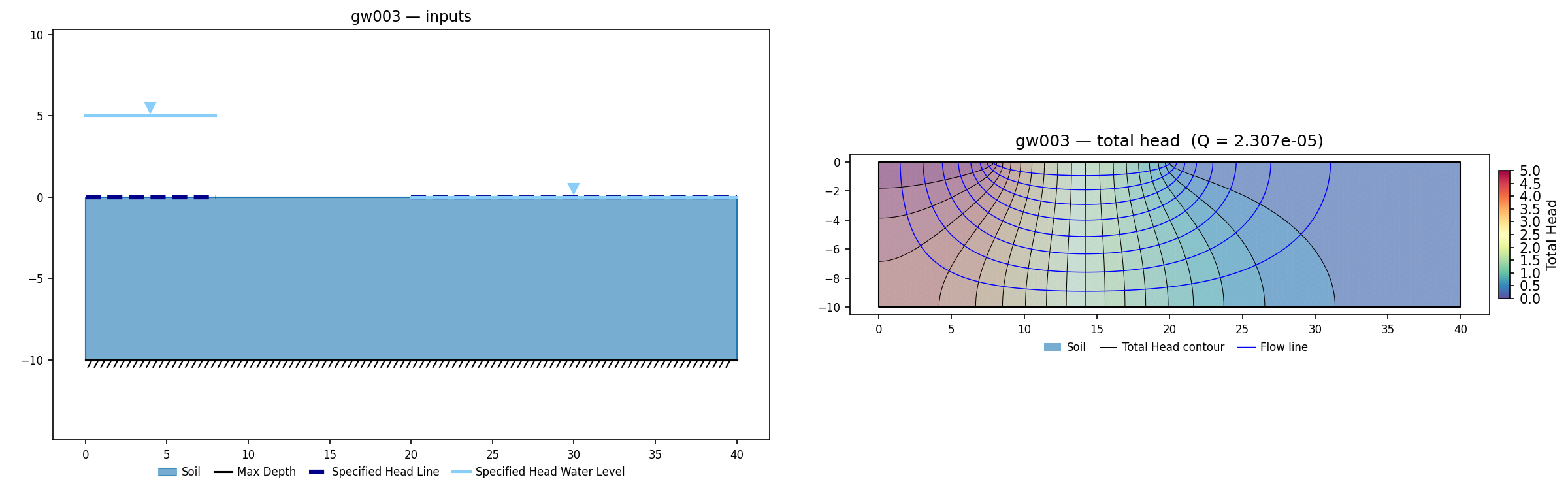
| 3 | Confined flow under dam foundation | built | gw003.xlsx. Rushton & Redshaw benchmark: head profiles under and beyond the dam within 0.08 m of the published chart everywhere. |
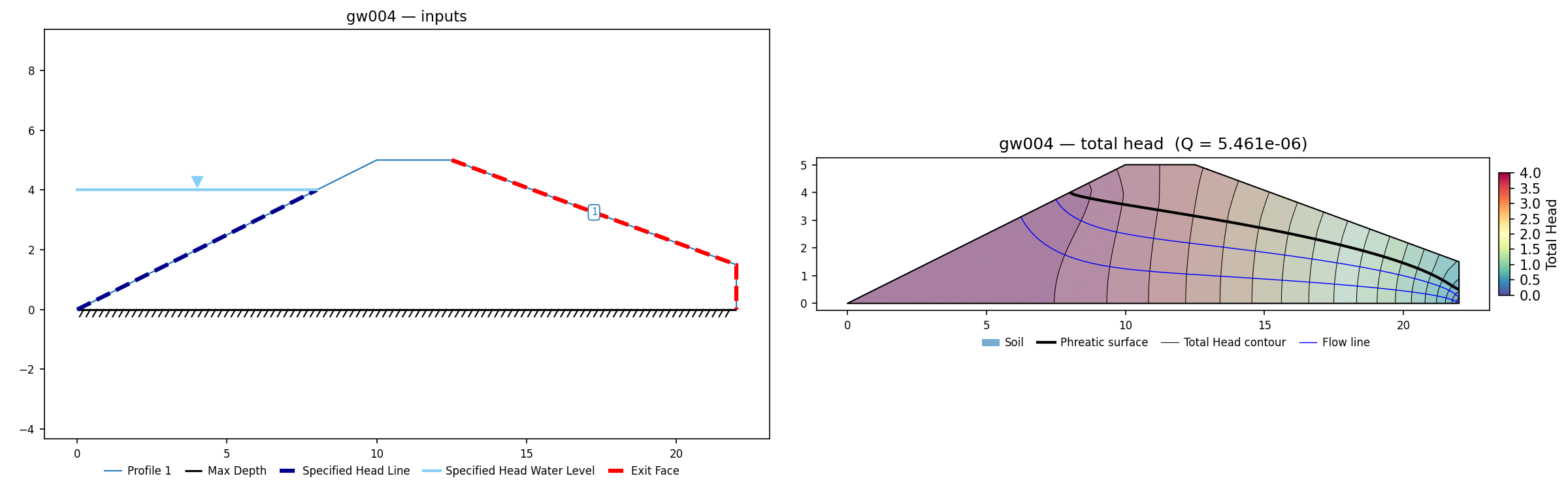
| 4 | Steady unconfined flow through earth dam | built | gw004.xlsx. Kozeny basic parabola: phreatic surface within 1–2% over the dam body; drain-tip height 0.50 vs Slide 0.442 / parabola 0.480 (the published pair itself spreads 9%). |
| 5 | Unsaturated flow behind an embankment | no lock possible | The manual publishes only qualitative pressure contours and flow lines against FLAC ("compared very well") — no numeric quantity exists to lock, and the geometry figure is unlabeled. |
| 6 | Steady-state seepage through saturated–unsaturated soils | built (4 of 5 cases) | gw006a (isotropic) / gw006b (9:1 anisotropy) / gw006c (core) / gw006e (seepage face). Fredlund & Rahardjo saturated–unsaturated dam, five cases sharing the same 12 m dam. The pressure-head profile along line 1-1 is a chart-only target (no tabulated value), so XSLOPE's own flowrate + total-head field are locked. Cases 2 and 5 reproduce the Slide/F&R curve almost exactly; cases 1 and 3 sit ~0.3–0.5 m high (the free-surface family, mesh- and fit-insensitive; the published Slide/Ref[1] themselves scatter ~1.5 m near the crest on case 3). Case 4 (steady infiltration) remains deferred on the flux-BC exit-face convergence. |
| 7 | Seepage within layered slope | built (caveat) | gw007.xlsx. Rulon & Freeze layered slope: 2.1×10⁻⁴ m/s infiltration on the crest — above the fine-sand ks — perches a water table on the fine lens and daylights as a slope-face spring. XSLOPE reproduces the stated water table (exits at el 0.30 at the toe) and the perched zone; Q = q·L = 1.68×10⁻⁴ locked. Every published target (Fig 7.4/7.7/7.8) is a chart curve with no tabulated value, so — as the methodology note allows for GW6/GW7 — only the flowrate is locked, with a head regression guarding the field. |
| 8 | Flow through ditch-drained soils | built (discrepancy) | gw008.xlsx. Gureghian (1981) ditch-drained aquifer — the corpus' exercise of the specified-flux boundary, since the problem is driven entirely by rainfall infiltration on the top surface. The flux boundary itself is verified exactly (total inflow = q·L; the confined response matches the closed form to six figures). The published contours cannot be reproduced from the manual's printed inputs: the recharge mound comes out ≈10× too small, and two independent hand calculations confirm the printed numbers cannot produce the published figure. Only the flowrate is locked. |
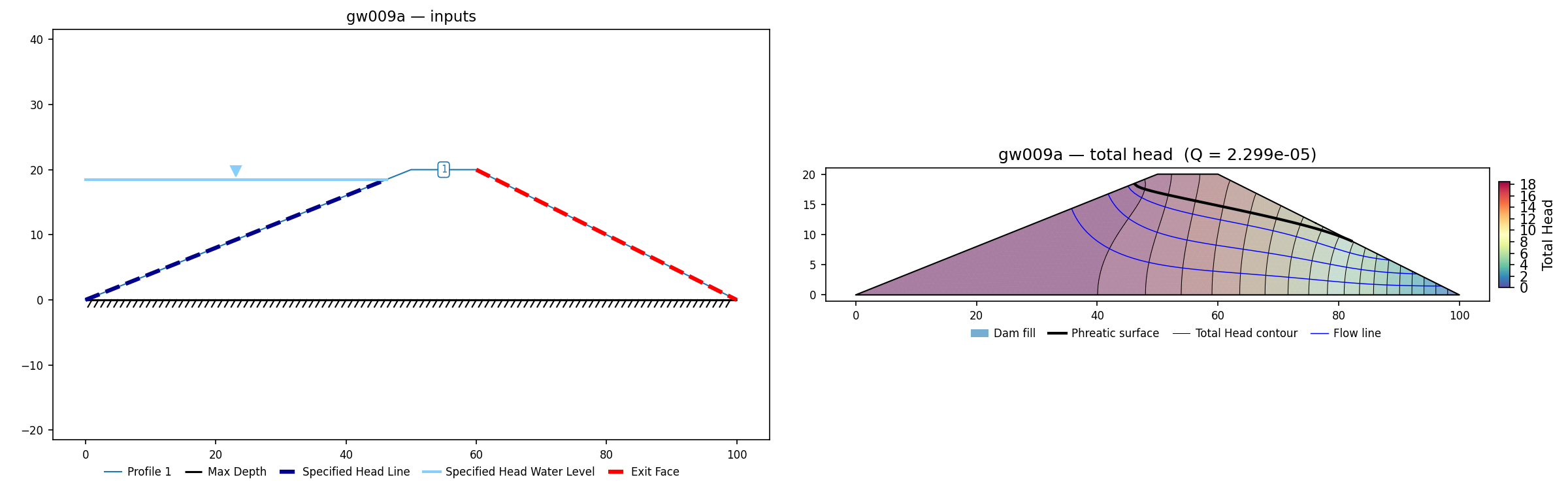
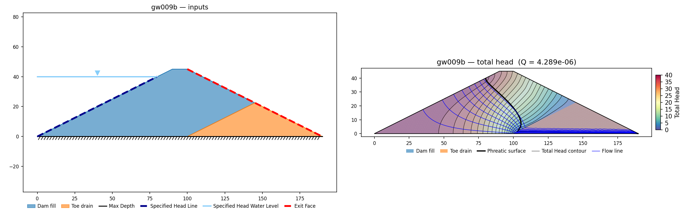
| 9 | Seepage through dam | built (both dams) | gw009a.xlsx (dam 1) · gw009b.xlsx (dam 2, toe drain). Bowles' dams via Chapuis et al. (2001). Dam 1: Q = 1.379×10⁻³ m³/(min·m) vs Slide 1.378×10⁻³ / SEEP/W 1.37×10⁻³ / Bowles flow nets 1.10–1.28×10⁻³. Dam 2: Q = 4.29×10⁻⁶ m³/(s·m) vs Slide / SEEP/W 4.23×10⁻⁶ / Bowles flow net 3.8×10⁻⁶ — all per second. Bowles (1984) Fig E9-2b pins the body k at 2.0×10⁻⁷ m/s, resolving a one-decade exponent slip in the Chapuis Fig 5 caption (2.0×10⁻⁶) and a min-vs-second units mislabel in the published flowrate. |
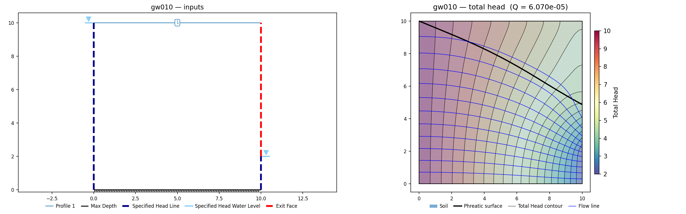
| 10 | Steady unconfined flow, van Genuchten permeability | built | gw010.xlsx. Clement et al. (1996): Q = 6.070×10⁻⁵ vs Slide 6.066×10⁻⁵ (+0.07%) / Clement 6.076×10⁻⁵; phreatic exit el. 4.87 vs Clement 4.8 / Slide 5.0. |
| 11 | Earth/rock-fill dam, Gardner permeability function | built (case 1 of 2, discrepancy) | gw011.xlsx. Zhang et al. (2001) homogeneous dam with the Gardner law (unsat=gard, a = 0.15, n = 6 as published). The free-surface release point comes out at el. 17.8 ± 0.15 against Slide 19.40 / ABAQUS 19.64 — about 1.6 m low, and the cause is not the conductivity model: the real Gardner law reproduces what van Genuchten and linear-front stand-ins gave (17.4). Mesh refinement (1.3k → 14.6k nodes) and the kr floor (1e-4 → 1e-8) both leave it unmoved. This is the one exit-face problem in the panel where XSLOPE releases low — the SEEP2D cross-check puts it on the same release point as SEEP2D everywhere else. Only the flowrate is locked; the release point is reported, not locked. Case 2 (zoned dam with foundation and toe drain) is not built. |
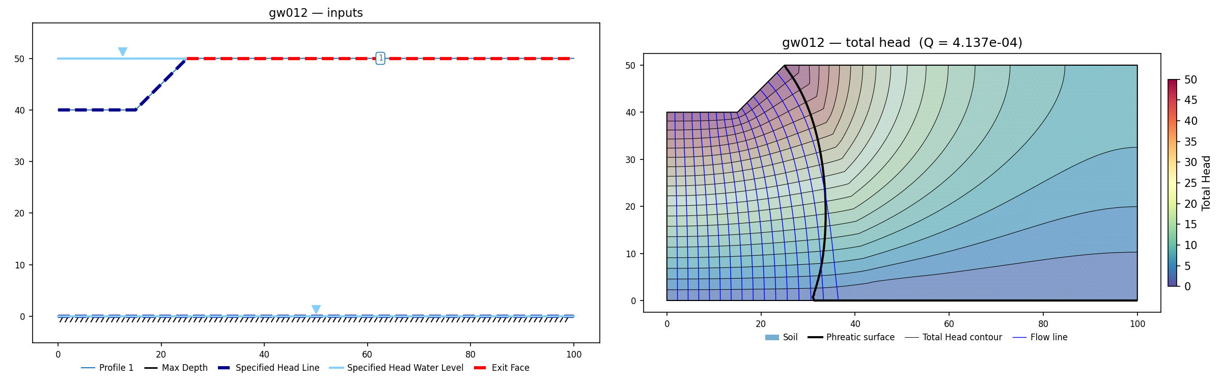
| 12 | Seepage from a trapezoidal ditch into a deep drainage layer | built | gw012.xlsx. Vedernikov: Q = 4.137×10⁻⁴ vs Slide 4.093×10⁻⁴ (+1.1%) / theory 4.0×10⁻⁴; flow-bulb half-width ≈42 vs Slide 41 / theory 40. |
| 13 | Seepage from a triangular ditch into a deep drainage layer | built | gw013.xlsx. Vedernikov: Q = 2.087×10⁻² vs Slide 2.050×10⁻² (+1.8%) / theory 2.0×10⁻². |
| 14 | Unsaturated soil column | blocked | Steady Gardner (1958) capillary profile (L = 1 m, ks = 10⁻⁷ m/s, ν = ±8.64×10⁻⁴ m/d = ±10⁻⁸ m/s, α = 1 m⁻¹). Confirmed blocked: the analytical profile is derived for the exponential Gardner law k = ks·e^(αψ) (the vendor RS2 model sets conductivity: Gardner, α = 1), which XSLOPE does not implement — its gard option is the power form kr = 1/(1 + a·ψⁿ). The manual publishes only Fig 14.3/14.4 charts (no tabulated Slide value), so with no matching law and nothing numeric to compare, the only lockable quantity is a 1-D through-flux the flux cross-check already verifies to machine precision. Blocked rather than tuned to a substitute curve. |
| 15 | 1-D consolidation, uniform initial excess pore pressure | blocked | Transient/consolidation — no transient solver |
| 16 | Pore pressure dissipation of stratified soil | blocked | Transient/consolidation |
| 17 | Transient seepage, earth fill dam with toe drain | blocked | Transient |
| 18 | Transient seepage through an earth fill dam | blocked | Transient |
| 19 | Transient seepage through an earth fill dam (II) | blocked | Transient |
| 20 | Transient seepage in a layered slope | blocked | Transient |
| 21 | Transient seepage through a fully confined aquifer | blocked | Transient |
Results
GW1: Shallow unconfined flow with rainfall
Input files: gw001.xlsx
Flow between two long parallel rivers 10 m apart (Haar 1990; the Dupuit–Forchheimer recharge problem), the manual's first specified-flux case. A 10 × 5 m block (base impermeable, ground surface at el 5) with river heads h₁ = 3.75 m on the left edge and h₂ = 3.0 m on the right, a uniform rainfall P = 2.5×10⁻⁶ m/s infiltrating the top, and k = 1×10⁻⁵ m/s. The recharge builds an internal free surface that mounds above both river levels; there is no daylighting seepage face, so the top edge is declared both the flux boundary and an (inactive) exit face — the device that puts the solver on the unsaturated free-surface path the internal mound needs. The free-surface position is set by mass balance, independent of k and of the unsaturated model.
| Quantity | XSLOPE | Slide | Haar eqs 1.2–1.3 |
|---|---|---|---|
| x_a (crest position) | ≈ 4.1 | 4.06 | 3.98 |
| h_max (crest elevation) | 4.61 | 4.49 | 4.25 |
| Q (m³/s per m) | 2.500×10⁻⁵ | — | P·L = 2.5×10⁻⁵ |
The mound crest lands within ~0.05 m of Slide in position and ~0.12 m in height — XSLOPE sits a touch above Slide, the same slightly-high free-surface bias the SEEP2D cross-check documents across this panel; both finite-element solutions sit above Haar's Dupuit closed form, which neglects the vertical flow the FE models resolve near the crest. The flowrate lock is Q = P·L = 2.5×10⁻⁵ (exact by construction, since all the rain enters and drains to the rivers); a head regression at three interior stations guards the mound shape, which the flux total alone does not.
GW2: Flow around cylinder
Input files: gw002.xlsx
Confined potential flow past a cylinder (Streeter's closed form; Desai & Kundu's finite elements): a half-domain 8 × 4 m with a semicircular notch of radius 1 m at the bottom center and fixed heads of 1.0 and 0.0 on the vertical edges. The domain is fully saturated, and the head field in homogeneous confined flow is independent of the conductivity, so the problem is determined by geometry and boundary heads alone.
| Point | XSLOPE | Slide | Closed form | Desai & Kundu |
|---|---|---|---|---|
| (4, 1) | 0.500 | 0.500 | 0.500 | 0.500 |
| (4.5, 0.866) | 0.381 | 0.381 | 0.375 | 0.378 |
| (5, 0) | 0.263 | 0.263 | 0.250 | 0.277 |
| (6, 0) | 0.202 | 0.203 | 0.188 | 0.213 |
| (8, 0) | 0.000 | 0.000 | −0.031 | 0.000 |
The two finite-element solutions agree with each other within 0.0013 m everywhere; both depart from the closed form near the downstream edge, where the analytical solution assumes an infinite domain (its −0.031 at the finite model's zero-head boundary measures that idealization, not an error). Flowrate is locked as a regression value.
GW3: Confined flow under a dam foundation
Input files: gw003.xlsx
The classic flow-net problem (Rushton & Redshaw): a 40 × 10 m soil block with head 5 m on the ground surface upstream of the dam (x = 0–8), head 0 downstream (x = 20–40), and the dam base impervious between them.
| Station (line 1-1, y = −4) | XSLOPE | Rushton & Redshaw / Slide |
|---|---|---|
| x = 0 | 4.47 | 4.50 |
| x = 10 | 3.40 | 3.45 |
| x = 14 | 2.44 | 2.47 |
| x = 20 | 1.05 | 1.05 |
| x = 30 | 0.19 | 0.20 |
| x = 40 | 0.08 | 0.07 |
Heads along both published profile lines fall within 0.08 m of the chart everywhere (Slide's markers coincide with Rushton & Redshaw's); the vertical profile on line 2-2 (x = 20) spans 0.17–1.30 m against the published 0.24–1.30 m.
This problem is solved on a finer mesh than the rest of the panel (target_size 0.1
rather than 0.4) because of the singularity at (20, 0), where the impervious dam base
meets the zero-head boundary. The head gradient is unbounded at that corner, so the
solution converges slowly in its immediate neighbourhood — the top of line 2-2 sits
right on top of it — while the rest of the domain is well resolved at any mesh size.
A coarse mesh reports a plausible number there for the wrong reason.
GW4: Steady unconfined flow through an earth dam
Input files: gw004.xlsx
Free-surface seepage through a small dam with a toe drain, against Kozeny's basic parabola: reservoir head 4 m on the upstream face, a seepage exit face on the downstream slope and drain end. The free-surface shape is independent of k.
| Quantity | XSLOPE | Slide | Kozeny parabola |
|---|---|---|---|
| Phreatic el. at x = 14 | 2.88 | — | 2.81 |
| Phreatic el. at x = 18 | 2.03 | — | 2.02 |
| Phreatic el. at x = 20 | 1.43 | — | 1.47 |
| y₁ at the drain | 0.50 | 0.442 | 0.480 |
The solved phreatic surface tracks the parabola within 1–2% across the dam body. At the drain tip the published values themselves spread 9% (Slide's measured 0.442 vs the parabola's 0.480), and the parabola is an idealization exact only at the drain; XSLOPE's 0.50–0.53 across a mesh refinement (Q changing 2%) sits just above that band. The flowrate lock (5.46×10⁻⁶ m³/s) exceeds the idealized k·y₁ = 4.80×10⁻⁶ because the parabola underestimates entry-face flow.
GW9: Seepage through dam
Input files: gw009a.xlsx (dam 1) · gw009b.xlsx (dam 2, toe drain)
Bowles' homogeneous dam, the flow-net textbook example re-solved numerically by Chapuis, Chenaf & Bowles (2001) and by Slide: base 100 m, crest 10 m at el. 20 (2.5:1 upstream, 2:1 downstream), reservoir head 18.5 m, ks = 6.67×10⁻⁶ m/s with the manual's printed 8-point unsaturated conductivity table, fit here by a Mualem–van Genuchten curve (α = 0.2835, n = 2.765).
| XSLOPE | Slide | SEEP/W (fine) | Bowles (flow nets) | |
|---|---|---|---|---|
| Q, m³/(min·m) | 1.379×10⁻³ | 1.378×10⁻³ | 1.37×10⁻³ | 1.10–1.28×10⁻³ |
Dam 2 — Bowles' dam with a toe drain (Bowles 1984, Example 9-2 / Fig E9-2b, p. 248; Slide manual §9.2, Fig 9.5; Chapuis et al. 2001, Fig 5). Base 190 m; crest 10 m wide at el. 45; symmetric 2:1 faces (upstream and downstream horizontal runs 90 m each); reservoir head 40 m. A coarse toe drain (ks = 1.0×10⁻⁴ m/s) fills the downstream-toe triangle (100, 0)–(190, 0)–(145, 22.5) — base 90 m, apex at mid-height of the downstream slope. The body's saturated conductivity is ks = 2.0×10⁻⁷ m/s, carrying the dam-1 unsaturated k(u) curve.
| XSLOPE | Slide | SEEP/W (2328 el.) | Bowles (flow net) | |
|---|---|---|---|---|
| Q, m³/(s·m) | 4.29×10⁻⁶ | 4.23×10⁻⁶ | 4.23×10⁻⁶ | 3.8×10⁻⁶ |
XSLOPE matches the two numerical benchmarks to 1.4% and Bowles' flow net to its graphical accuracy. Note the units: dam 2 is worked per second (Bowles solves it in cm/s), where dam 1 was per minute.
Provenance. The body conductivity comes straight from Bowles (1984), Example 9-2, Fig E9-2b: the figure prints k = 2×10⁻⁵ cm/s = 2.0×10⁻⁷ m/s, and its flow net (n_f/n_d = 1.9/4) gives q = k·h·n_f/n_d = 2.0×10⁻⁷ × 40 × 0.475 = 3.8×10⁻⁶ m³/(s·m) as an independent hand-check. (Bowles' printed answer, 3.8×10⁻² m³/(s·m), applies the cm→m factor the wrong way in that same line; the conductivity, head, and flow net are unambiguous.) Two errata in the secondary sources are resolved by the figure:
- Body k. The 2.0×10⁻⁶ m/s in the Chapuis et al. (2001) Fig 5 caption is one decade high — a −6/−7 exponent slip. Bowles' value is 2.0×10⁻⁷ m/s, and the Slide manual's own Fig 9.6 chart draws the earth-dam curve at ≈2×10⁻⁷.
- Flowrate units. The published Q, tabulated as m³/(min·m) beside dam 1, is actually m³/(s·m). Bowles 3.8×10⁻⁶ and Chapuis's SEEP/W and Slide 4.23×10⁻⁶ are all per second, and agree because all three used k ≈ 2×10⁻⁷ m/s.
Run at the caption's 2.0×10⁻⁶ m/s, XSLOPE returns 3.97×10⁻⁵ m³/(s·m) — an order of magnitude above the published value (Q is nearly linear in k), the exponent slip made visible. The lock uses XSLOPE's own Q at Bowles' conductivity, 4.29×10⁻⁶ m³/(s·m).
Vendor check. The RS2 Groundwater Verification set ships only groundwater #009_01.fez
(dam 1, no drain); the Slide manual's Groundwater#09_2.sli is not in the distributed model
set. Neither is needed — Bowles (1984) fixes the conductivity directly.
GW10: Steady unconfined flow, van Genuchten permeability
Input files: gw010.xlsx
Clement, Wise, Molz & Wen (1996)'s unconfined square domain, the manual's designated
van Genuchten test: a 10 × 10 m block with head 10 on the left edge, tailwater 2 on the
right, an exit face above the tailwater, and vG conductivity (α = 0.64, n = 4.65,
ks = 1.1574×10⁻⁵ m/s) — an exact capability match for the solver's vg option.
| XSLOPE | Slide | Clement et al. | |
|---|---|---|---|
| Q (m³/s per m) | 6.070×10⁻⁵ | 6.066×10⁻⁵ | 6.076×10⁻⁵ |
| Phreatic exit elevation | 4.87 | 5.0 | 4.8 |
The manual's "seepage face" column tabulates the phreatic exit elevation (both published figures show the free surface exiting near el. 4.9–5.0), not a face length. Only the tailwater-2 case carries published numbers and is locked.
GW12 / GW13: Ditch seepage into a deep drainage layer (Vedernikov)
Input files: gw012.xlsx (trapezoidal) · gw013.xlsx (triangular)
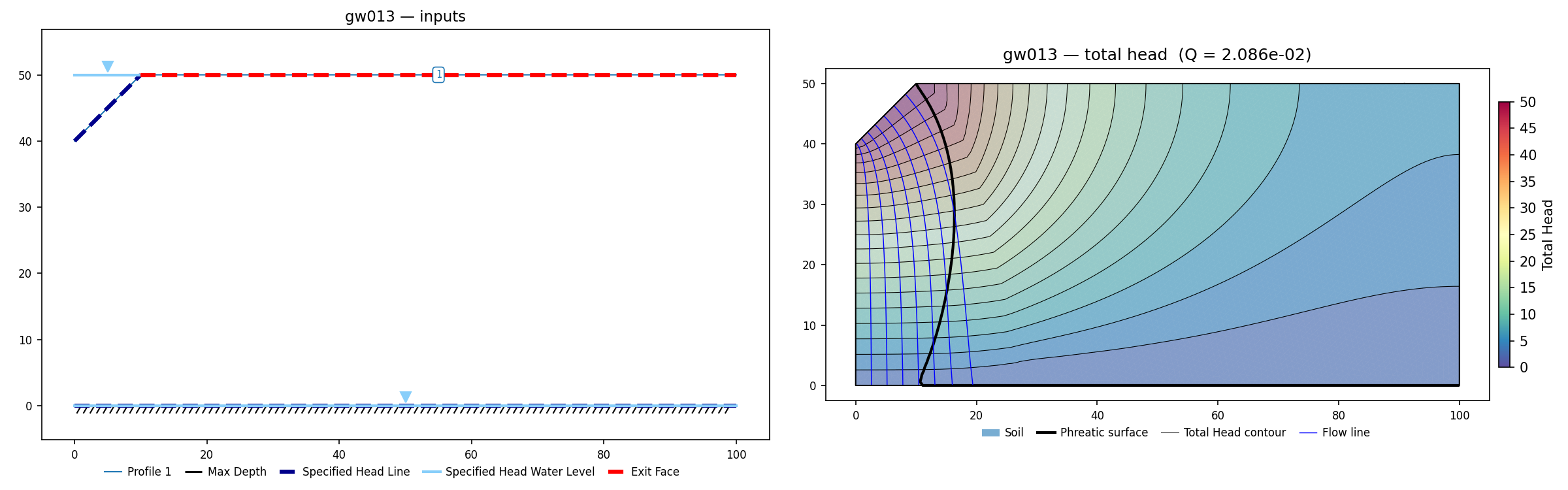
Vedernikov's closed-form solutions for steady seepage from a channel into a deep drainage layer, modeled as half-domains by symmetry with the ditch perimeter at head 50 and the deep drain as head 0 on the base. The seepage detaches below the ditch and descends as a bulb whose width the theory predicts.
| XSLOPE | Slide | Vedernikov | |
|---|---|---|---|
| Trapezoidal: Q per half | 4.137×10⁻⁴ | 4.093×10⁻⁴ | 4.0×10⁻⁴ |
| Trapezoidal: bulb half-width | ≈42 | 41 | 40 |
| Triangular: Q per half | 2.087×10⁻² | 2.050×10⁻² | 2.0×10⁻² |
The detached-bulb iteration converges cleanly at 1,500 free-surface iterations (the
max_iter tag key); the default 400 is not enough for these geometries.
GW6: Steady-state seepage through saturated–unsaturated soils
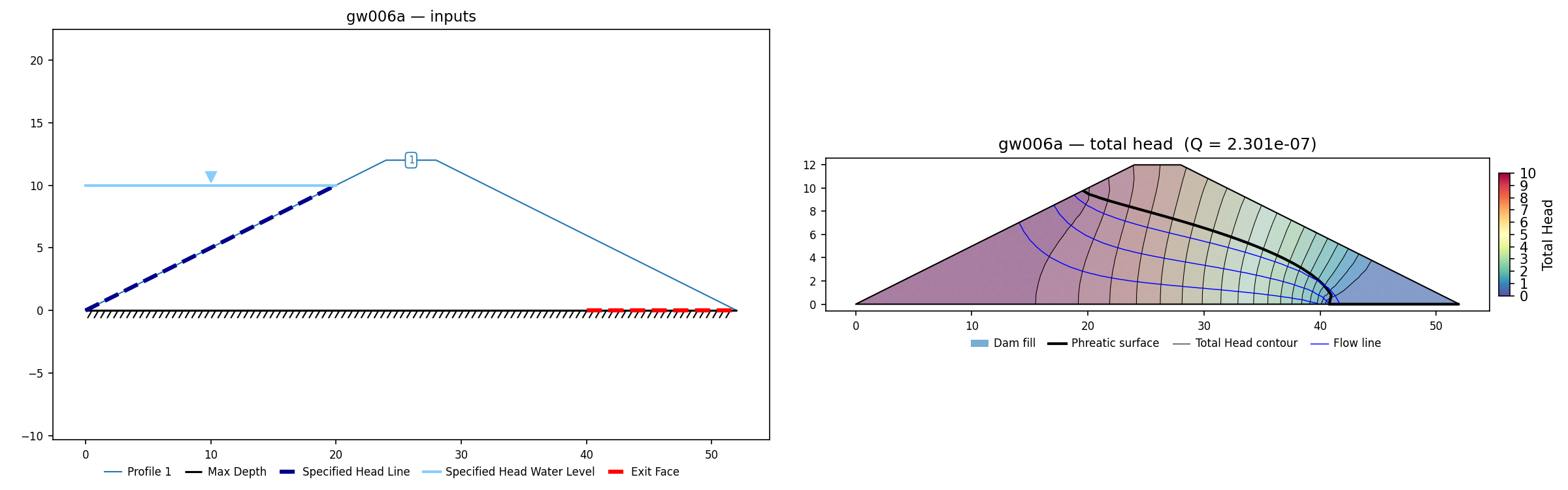
Input files: gw006a.xlsx (case 1, isotropic) / gw006b.xlsx (case 2, 9:1 anisotropy) / gw006c.xlsx (case 3, core) / gw006e.xlsx (case 5, seepage face)
This manual problem runs the same 12 m dam through five cases. The published target in every
case is the pressure-head profile along line 1-1 (the crest centerline, x = 26) — a chart
curve (Figs 6.6 / 6.9 / 6.14 / 6.23) with no tabulated value — so, as the methodology note
allows for GW6/GW7, each case locks XSLOPE's own flowrate and total-head field. The case-2/3/5
material and boundary data were read verbatim from the vendor RS2 groundwater models
(groundwater #006_02/03/05.slw in the RS2 Groundwater zip): case 2's condx:1 condy:0.111111
(kₕ = 9e-7, k_v = 1e-7), case 3's 100×-lower core over the mesh's material-2 footprint (a
rectangle x ∈ [24, 28], y ∈ [0, 10]), and case 5's crest-plus-downstream-slope seepage face.
Case 1 — isotropic dam with a 12 m horizontal drain.
Fredlund & Rahardjo (1993)'s saturated–unsaturated earth dam (12 m high, symmetric 2:1 faces, reservoir at 10 m, a 12 m horizontal drain at the downstream toe), case 1: isotropic conductivity. The conductivity function is digitized from the manual's chart (ks = 10⁻⁷ m/s, air entry ≈ 9 kPa) and fit by a Mualem–van Genuchten curve; three fit variants move the answer by less than 3 cm, so the fit is not the controlling uncertainty. The published target is the pressure-head profile along the crest centerline, where Slide's and Fredlund & Rahardjo's curves coincide within 0.2 m.
| Elevation on the crest line | XSLOPE pressure head | Slide | F&R |
|---|---|---|---|
| 0 | 7.40 | 7.15 | ≈7.3 |
| 2 | 5.47 | 5.15 | ≈5.3 |
| 4 | 3.52 | 3.25 | ≈3.4 |
| 6 | 1.66 | 1.30 | ≈1.45 |
| 8 | −0.22 | −0.60 | ≈−0.45 |
The profile shape reproduces exactly; the whole curve sits 0.25–0.5 m above the published pair, insensitive to the conductivity fit and to mesh refinement. This is a family difference, not a solver error: run against SEEP2D (the original USACE/WES code) on the identical mesh, boundary conditions and unsaturated law, XSLOPE's free surface daylights at the same place — see the SEEP2D cross-check below. The regression locks XSLOPE's own values.
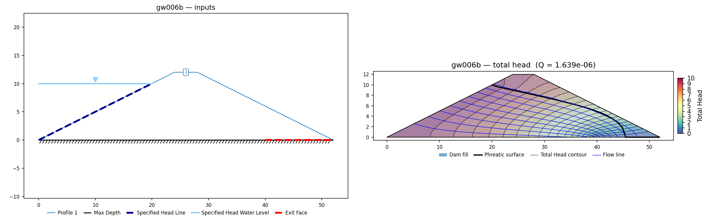
Case 2 — anisotropic dam (kₕ = 9 kᵥ) with the horizontal drain. The horizontal
conductivity is nine times the vertical (vendor condx:1 condy:0.111111, so kₕ = 9×10⁻⁷,
kᵥ = 10⁻⁷ m/s), which spreads the flow and lowers the phreatic surface; the unsaturated
relative shape is identical to case 1, so the same Mualem–vG fit is reused. Here XSLOPE
reproduces the published curve almost exactly:
| Elevation on line 1-1 | XSLOPE pressure head | Slide / F&R (Fig 6.9) |
|---|---|---|
| 0 | 6.52 | ≈6.5 |
| 2 | 4.74 | ≈4.7 |
| 4 | 3.19 | ≈3.2 |
| 6 | 1.79 | ≈1.85 |
| 8 | 0.42 | ≈0.4 |
Flowrate 1.639×10⁻⁶ m³/s per m (locked with the total-head field).
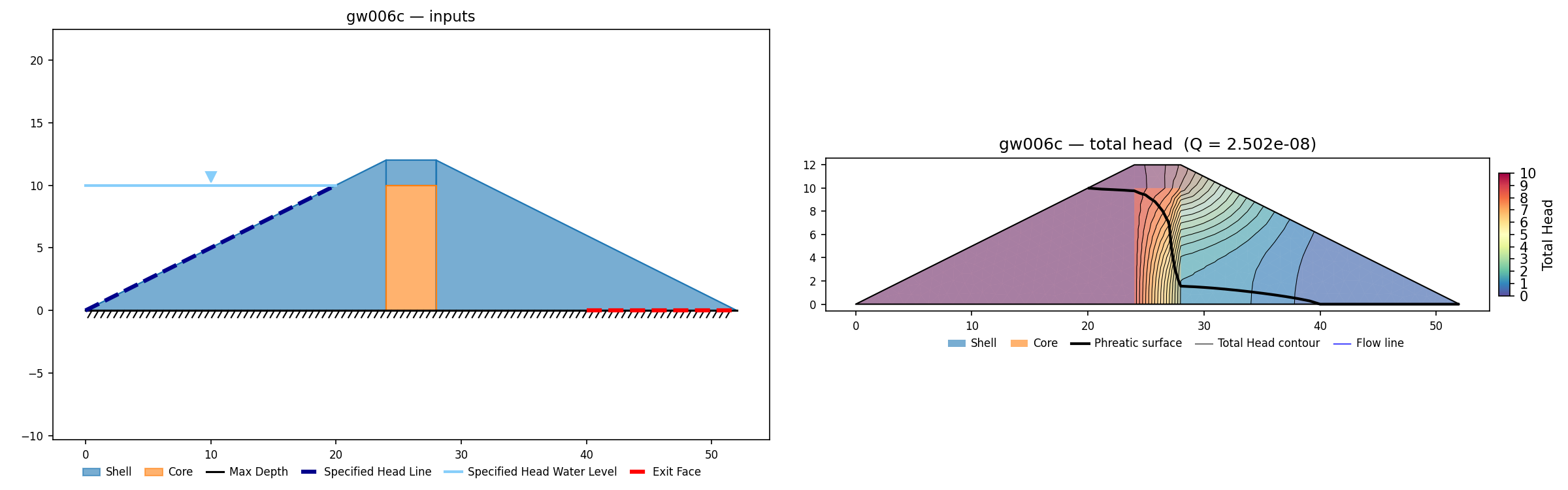
Case 3 — isotropic dam with a low-permeability core and the horizontal drain. A rectangular central core (x ∈ [24, 28], y ∈ [0, 10], read from the vendor mesh's material-2 footprint) with saturated k = 10⁻⁹ m/s — 100× lower than the 10⁻⁷ shell — is tiled into the dam as four non-overlapping polygons (three shell pieces + the core). The core forces almost the whole head drop across its 4 m width (Fig 6.13's crowded contours), throttling the flowrate to 2.502×10⁻⁸ m³/s per m. Along line 1-1 (now inside the core) XSLOPE reproduces the profile shape and sits at the high end of the published scatter:
| Elevation on line 1-1 | XSLOPE pressure head | Slide (Fig 6.14) | Ref[1] |
|---|---|---|---|
| 0 | 5.55 | ≈5.9 | ≈5.8 |
| 2 | 4.06 | ≈3.9 | ≈3.9 |
| 4 | 2.68 | ≈2.1 | ≈2.1 |
| 6 | 1.48 | ≈0.4 | ≈0.7 |
| 8 | 0.28 | ≈−1.2 | ≈−0.3 |
The published Slide and Ref[1] curves themselves diverge ~1.5 m near the crest; XSLOPE tracks the shape and sits above both up high — the same +0.5 m free-surface family as case 1. Locked at XSLOPE's own values.
Case 5 — isotropic dam with a downstream seepage face (no drain). The horizontal toe drain is replaced by the "unknown boundary condition": the crest and the whole downstream slope are a seepage face where the phreatic surface may daylight (vendor seepage-face nodes (22,11)→(50,1)). Without the drain the phreatic surface rides higher. XSLOPE again reproduces the published curve almost exactly:
| Elevation on line 1-1 | XSLOPE pressure head | Slide / F&R (Fig 6.23) |
|---|---|---|
| 0 | 8.29 | ≈8.4 |
| 2 | 6.35 | ≈6.4 |
| 4 | 4.39 | ≈4.5 |
| 6 | 2.45 | ≈2.5 |
| 8 | 0.50 | ≈0.55 |
Flowrate 1.686×10⁻⁷ m³/s per m (locked with the total-head field).
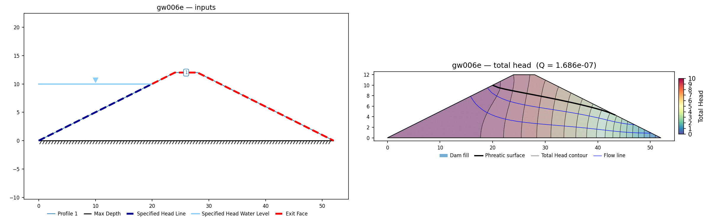
Case 4 (steady-state infiltration, a 10⁻⁸ m/s flux over the whole dam surface) stays deferred — the same flux-BC / exit-face convergence gap tracked elsewhere in this corpus.
GW7: Seepage within a layered slope
Input file: gw007.xlsx
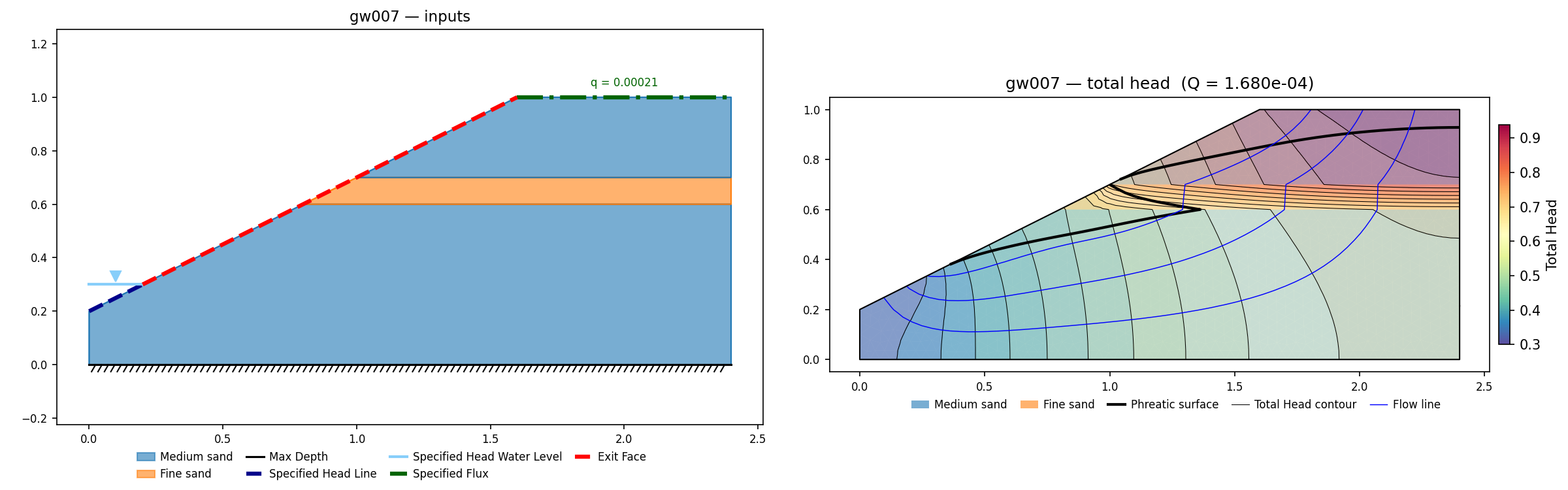
Rulon & Freeze's sandbox slope (after Fredlund & Rahardjo 1993): a medium-sand slope holding a thin fine-sand lens. Geometry from the vendor RS2 model (a 2.4 × 1.0 m box, a 2:1 downstream slope from the crest at (1.6, 1.0) to the toe at (0, 0.2), and the fine lens as the y = 0.6–0.7 band from the slope face to the right wall); conductivity curves from the manual's Fig 7.2, fit here by Mualem–van Genuchten (medium ks = 1.4×10⁻³ m/s, fine ks = 5.5×10⁻⁵ m/s). A uniform 2.1×10⁻⁴ m/s falls on the crest; the submerged toe is a tailwater head of 0.3 m; the rest of the slope is a seepage face; base and right wall are no-flow.
The infiltration rate exceeds the fine sand's saturated conductivity, so the recharge cannot drain vertically through the lens: it perches a water table on top of the fine band and sheds laterally to daylight as a slope-face spring — the physical result Rulon & Freeze observed. XSLOPE reproduces it: the perched saturated zone above the lens (the crowded head contours across the low-k band), the free surface daylighting on the slope, and the main water table exiting at el 0.30 at the toe — the "0.3 m from the toe" the manual reports.
| Quantity | XSLOPE | Slide / Rulon & Freeze |
|---|---|---|
| water table at the toe | el 0.30 | 0.3 m (stated) |
| Q, m³/s per m | 1.680×10⁻⁴ | q·L = 1.68×10⁻⁴ |
Every published target is a chart curve — the water table (Fig 7.4) and the total-head profiles along lines 1-1 and 2-2 (Figs 7.7, 7.8) — with no tabulated number, the same situation the methodology note flags for GW6/GW7. So only the flowrate is locked (Q = q·L, exact by construction on the flux boundary), with a three-station head regression guarding the solved field. The conductivity fit shifts the unsaturated detail but not the flowrate or the perched-table topology.
GW8: Flow through ditch-drained soils
Input file: gw008.xlsx
A ditch-drained two-layer aquifer after Gureghian (1981), and the corpus' exercise of the specified-flux boundary — the whole problem is driven by rainfall infiltration on the ground surface, so it cannot be posed at all without one. A half-drain spacing of 1.0 m over an impermeable base at 0.5 m depth; a coarse Soil A in the lowest 0.1 m (k = 1.11×10⁻³ m/s, Gardner a = 1000, n = 4.5) beneath a finer Soil B (k = 1.11×10⁻⁴ m/s, a = 2777.7, n = 4.2); a uniform infiltration of 4.4×10⁻⁶ m/s on the top; the water-free ditch as a seepage face on the left wall; base and right-hand symmetry edge no-flow.
The flux boundary behaves exactly. Total applied inflow is q·L = 4.400000×10⁻⁶ at every mesh size; the confined form of the same model (fix the base, remove the seepage face) produces a head rise of 0.016252 m against the one-dimensional hand calculation q·(0.4/kB + 0.1/kA) = 0.016252 m, agreeing to six figures; and the computed suction in the unsaturated zone lands on the Gardner gravity asymptote — with kr = q/ks = 0.0396, the law gives ψ* = 0.323 m, against a computed −0.315 m. Reversing the sign of q inverts the response antisymmetrically. The reported flowrate is q·L = 4.400000×10⁻⁶ to six figures at every mesh size tested, from 243 to 14 867 nodes.
The published contours, however, do not follow from the printed inputs.
| XSLOPE | Slide / Gureghian (Figs 8.3, 8.4) | |
|---|---|---|
| total head | 0.000 – 0.186 m | 0.05 – 0.29 m |
| pressure head, unsaturated zone | to −0.315 m | −0.10 to −0.20 m |
| water table at the symmetry edge | 0.025 m | ≈0.25 m |
The mound is about ten times too small, and this is not a solver error. A Dupuit calculation on the layered aquifer gives an upper bound on the mound of √(q/kA) = 0.063 m — generous, because it credits only the saturated transmissivity — which is already four times below the published 0.25 m. The printed infiltration and the printed conductivities cannot produce the published water table, whatever code solves them. Scaling q/k by ten reproduces the charts closely (water table 0.256 m, minimum pressure head −0.162 m), which suggests the manual's "4.4×10⁻⁶" may be a per-node discharge on its own mesh rather than a distributed flux — but that is a conjecture, and the input file carries the printed values, untuned.
Only the flowrate is locked, on tri3: the total inflow is the one quantity here that is exact by construction. No head lock is taken, because locking XSLOPE's own head field would enshrine numbers the manual contradicts.
GW11: Earth/rock-fill dam, Gardner permeability function
Input file: gw011.xlsx
A 45 m homogeneous earth/rock-fill dam after Zhang et al. (2001), and the manual's dedicated test of the Gardner relative-conductivity function, \(k_r = 1/(1 + a\,\psi^n)\), with the published \(a\) = 0.15 and \(n\) = 6. Crest 17 m, upstream run 89.1 m, downstream run 76.9 m, impermeable base; reservoir at el. 40 m, no tailwater; the whole downstream slope is an exit face. The published quantity is the release point — the elevation at which the free surface daylights on the downstream face.
| release point | |
|---|---|
XSLOPE (Gardner, target_size = 1.0) |
17.90 m |
| Slide | 19.397 m |
| ABAQUS (Zhang et al.) | 19.64 m |
XSLOPE releases about 1.6 m low, and this is an open discrepancy rather than a resolved one.
The unsaturated conductivity model is not the cause. This problem exists to test Gardner, and the real Gardner law reproduces what van Genuchten and linear-front stand-ins gave (≈17.4 m) before it was implemented. Nor is it discretization or the relative-conductivity floor:
target_size |
nodes | release point |
|---|---|---|
| 2.0 | 1,338 | 17.79 m |
| 1.0 | 5,317 | 17.90 m |
| 0.6 | 14,621 | 17.76 m |
There is no trend with refinement, and at the finest mesh the next face node above the release point sits at 18.06 m — still 1.3 m below Slide, so the gap is not a nodal-resolution artifact. The release point is identical to three decimals for \(k_{r,\min}\) = 10⁻⁴, 10⁻⁶ and 10⁻⁸.
Two notes on reading the manual. Its text gives the downstream slope as 1:1.171, but the printed dimensions on Fig. 11.1 give 76.9/45 = 1.709 — a digit transposition. The figure's dimensions are used here (they also agree with a direct measurement of the plate), and they are the more favourable read: the text's slope releases at 16.54 m, lower still. Separately, \(k_s\) is not printed for this case; because the dam is homogeneous the free-surface position is independent of \(k_s\), so it does not affect the published target, but it does set the discharge — which is why the regression tag below locks XSLOPE's own flowrate rather than a published one.
GW11 is the single exit-face problem in this panel where XSLOPE releases low. The SEEP2D cross-check below puts XSLOPE on the same release point as the original USACE code on every other exit-face problem, which is what makes this one worth flagging rather than filing as a family-wide convention difference. Case 2 of the manual's problem (the zoned dam with a foundation and toe drain) is not built.
The SEEP2D cross-check: where does the free surface daylight?
Several problems on this page reproduce a published profile in shape but sit a little high, and the free surface on a steep exit face looked like the common thread. The question is whether XSLOPE places the release point — the top of the saturated seepage face, where the phreatic surface daylights — differently from other codes.
It is answerable directly, because XSLOPE's seepage solver is in the SEEP2D family. The
original USACE/WES SEEP2D Fortran program is run on the identical tri3 mesh, the
identical boundary conditions and the identical unsaturated law (SEEP2D's iuntyp:
linear front, or van Genuchten — both codes use the same Mualem–van Genuchten form, so
α and n carry straight across), and the two solutions are compared node for node. The
harness is benchmarks/run_seep2d_compare.py --gw.
| problem | law | release point, XSLOPE | release point, SEEP2D | head RMS | head range |
|---|---|---|---|---|---|
| gw004 | linear front | 0.500 | 0.500 | 0.0004 | 0–4 |
| gw006a | van Genuchten | 0.000 | 0.000 | 0.0000 | 0–10 |
| gw009a | van Genuchten | 8.846 | 8.462 | 0.0026 | 0–18.5 |
| gw010 | van Genuchten | 4.872 | 4.872 | 0.0006 | 2–10 |
| gw012 | linear front | face dry | face dry | 0.034 | 0–50 |
| gw013 | linear front | face dry | face dry | 0.070 | 0–50 |
The release point agrees. It is identical on gw004, gw006a and gw010; both codes leave the face fully drained on gw012 and gw013; and gw009a differs by 0.385 — a single element at that mesh. The head fields agree to a relative RMS of order 10⁻⁴ throughout. XSLOPE does not release low. Where this corpus sits above a published profile, the difference is between the SEEP2D family and the reference code's exit-face convention, not an XSLOPE defect — so those problems are locked on XSLOPE's own values with the offset reported, rather than tuned.
One open item came out of the same run. On the van Genuchten problems the total
discharge reads 3.5–4.7% below SEEP2D (gw009a 2.299×10⁻⁵ vs 2.412×10⁻⁵; gw010
6.070×10⁻⁵ vs 6.294×10⁻⁵) even though the heads agree to 10⁻⁴ — while the linear-front
problems agree on discharge to better than 0.15%. The split follows the unsaturated law
exactly, and it is not XSLOPE's kr floor: dropping kr_min from 10⁻⁴ to zero leaves
the discharge unchanged to six figures. Since the head field is right and only the
integrated flux differs, the likely cause is where each code evaluates the strongly
nonlinear kr(ψ) when it forms an element's conductivity. That is being tracked
separately; it does not affect pore pressures or stability, which read the head field.
The specified-flux boundary, against SEEP2D
The same harness verifies the
specified-flux (Neumann) boundary,
because SEEP2D supports one natively. It is entered as flowrate cards — a boundary segment
and a flux — and SEEP2D forms its own consistent nodal loads from them (seep2d.f, the
nflcd block: fx(i) += ½·L·q at each end of the segment, and it sets the flux flags itself).
So SEEP2D is handed the raw segment and flux, never XSLOPE's assembled vector, and the two
codes' assemblies are compared rather than one being fed the other's answer.
The test problem is a confined rectangle, 10 × 4, isotropic k = 2, with a fixed head on one side and a uniform inflow q on the other, no-flow above and below. One-dimensional Darcy gives the head exactly: h(x) = q(L − x)/k, with total inflow q·H.
| XSLOPE | SEEP2D | |
|---|---|---|
| max abs. error vs the exact solution | 2.5×10⁻¹⁹ | 5.0×10⁻⁹ |
| total inflow (exact: 1.760000×10⁻⁵) | 1.760000×10⁻⁵ | 1.759800×10⁻⁵ |
| max abs. difference, XSLOPE − SEEP2D | -- | 5.0×10⁻⁹ (2.3×10⁻⁴ of the head range) |
XSLOPE reproduces the closed form to machine precision, and matches SEEP2D to that code's own iteration tolerance.
Machine-precision agreement on the head field — not merely on the total — is the check that matters. A linear head field only satisfies A·h = f when f is the consistent load vector, so an incorrect distribution along an edge (½, ½, 0 across a quadratic edge, say) would still sum to q·L and pass a total-flux check while breaking the solution. It does not. The quadratic weights (⅙, ⅙, ⅔ at corner, corner and midside) are verified the same way, and a zero flux reproduces the no-flux answer bitwise.
Methodology
Same rules as the Slide2 corpus: problems are built from the manual's tabulated
data and coordinate-labeled figures; where a figure is unlabeled, geometry is extracted by
axis-calibrated pixel measurement and validated against printed solution quantities; every built
problem is locked into run_tests.py via test tags. Seepage problems compare flow rates,
phreatic-surface positions, and head/pressure profiles rather than factors of safety. Two tag
types carry the locks: type=seep (flowrate, live mesh + solve at target_size) and
type=seep_head (solved total head at named x:y:h points, interpolated from the four nearest
nodes). Where a problem's published answer is itself a chart curve (GW6/GW7), a
tolerance-banded profile lock is planned but not yet implemented.