Ordinary Method of Slices (OMS)

The Ordinary Method of Slices (also known as the Swedish Method) is one of the simplest limit equilibrium techniques used for slope stability analysis. The factor of safety can be calculated directly without iteration. The key assumption for the OMS method is that the side forces can be neglected, meaning interslice shear and normal forces cancel out and are excluded from equilibrium considerations. Because it ignores interslice forces entirely and satisfies only overall moment equilibrium, OMS is the least accurate of the procedures in xslope — it can be markedly conservative on effective-stress surfaces with high pore pressures — and is included primarily as a historical and teaching baseline rather than for design. The forces on the slice are as follows:

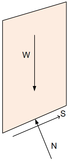
Further, only moment equilibrium about the center of the slip circle is enforced:

\(\sum M = 0\)

Force equilibrium in the horizontal and vertical directions is not satisfied.

Basic Formulation

To solve for the factor of safety, we need to consider the forces acting on the slice:

\(W\) = weight of the slice
\(\alpha\) = inclination of the base of the slice
\(\Delta \ell\) = length of the slice base
\(S\) = shear force on the base of the slice = \(c \Delta \ell + N \tan \phi\)
\(c\) = cohesion
\(\phi\) = friction angle
\(N\) = normal force on the base of the slice
\(u\) = pore water pressure

The general expression for the factor of safety \(FS\) is:

\(FS = \dfrac{\sum (c \Delta \ell + N \tan \phi)}{\sum W \sin \alpha} \qquad (1)\)

Summing forces perpendicular to the base, the normal force on the base is:

\(N = W \cos \alpha\)

Therefore, we can rewrite (1) as:

\(FS = \dfrac{\sum (c \Delta \ell + W \cos \alpha \tan \phi)}{\sum W \sin \alpha}\)

If \(\phi = 0\), the expression simplifies to:

\(FS = \dfrac{\sum c \Delta \ell}{\sum W \sin \alpha}\)

which is the same equation used in the Swedish method and the log-spiral method under the same assumptions.

To use effective stress parameters \(c', \phi'\), and effective normal stress \(\sigma'\), the expression becomes:

\(S = c' \Delta \ell + N' \tan \phi\)

\(N' = N - u \Delta \ell = W \cos \alpha - u \Delta \ell\)

\(S = c' \Delta \ell + (W \cos \alpha - u \Delta \ell) \tan \phi\)

\(FS = \dfrac{\sum (c' \Delta \ell + (W \cos \alpha - u \Delta \ell) \tan \phi')}{\sum W \sin \alpha} \qquad (2)\)

Alternate (Preferred) Formulation

This equation for FS can produce unconservative results, including negative normal stresses under high pore pressures. The following formulation is preferred. First, we define the effective weight as follows:

\(W' = W - u b, \quad \text{where} \quad b = \Delta \ell \cos \alpha\)

\(W' = W - u \Delta \ell \cos \alpha\)

Then:

\(N' = W' \cos \alpha = (W - u \Delta \ell \cos \alpha) \cos \alpha\)

\(N' = W \cos \alpha - u \Delta \ell \cos^2 \alpha\)

Substituting into (2):

\(F = \dfrac{\sum \left[ c' \Delta \ell + (W \cos \alpha - u \Delta \ell \cos^2 \alpha) \tan \phi' \right]}{\sum W \sin \alpha} \qquad (3)\)

This is the preferred formulation for OMS.

Complete Formulation

For a complete implementation of the Ordinary Method of Slices, we need to consider some additional forces to the slice. The full set of forces acting on the slice are as follows:

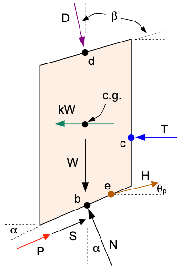
Where:

\(D\) = distributed load resultant force
\(\beta\) = inclination of the distributed load (perpendicular to slope)
\(kW\) = seismic force for pseudo-static seismic analysis
\(c.g.\) = center of gravity of the slice
\(P\) = reinforcement force at point \(r\) on the base of the slice
\(\psi\) = angle of the reinforcement force from horizontal
\(T\) = tension crack water force
\(H\) = pile/pier force at point \(e\) on the failure surface
\(\theta_p\) = angle of pile force from horizontal (positive = counterclockwise/upward)
\(L\) = line load at point \(f\) on the top of the slice
\(\delta\) = angle of the line load from horizontal (default \(-90°\) = straight down)

The rest of the forces are the same as before.

⚠ TODO (figures): the force diagram above must be redrawn in LibreOffice Draw — show the reinforcement force \(P\) at a general angle \(\psi\) (not tangent to the base) applied at point \(r\), and add the line load \(L\) at angle \(\delta\) applied at point \(f\) on the top of the slice.

The distributed load resultant force \(D\) is calculated from the distributed load input which is defined as a stress along the top of the slope. It is assumed to act perpendicular to the slope, therefore the inclination of the distributed load from a vertical line is equal to the slope angle, \(\beta\). The distributed load acts through point \(d\) which is often the center of the slice, but it can be offset from the center, depending on how the distributed load is defined.

The seismic force \(kW\) is calculated as a horizontal pseudo-static force acting on the slice through the center of gravity of the slice. It is assumed to act in the direction of sliding. It is equal to the seismic coefficient \(k\) multiplied by the weight of the slice \(W\). The seismic coefficient is a user-defined input, depending on the seismic conditions of the site.

The reinforcement force \(P\) is applied at the point \(r = (x_r, y_r)\) where a reinforcement line crosses the base of the slice, in a direction resisting sliding. Its magnitude is the available tensile capacity of the line at the crossing point, interpolated from the line's capacity envelope (tensile strength, pullout development, and end anchorage — see the reinforcement page). Its direction depends on the line's Dir setting in the input:

• Tangent (the default): flexible reinforcement (geosynthetics) is assumed to bend with the sliding mass so the force acts parallel to the base of the slice, i.e. \(\psi = \alpha\).
• Axial: rigid reinforcement (soil nails, tiebacks) carries the force along its own axis, so \(\psi\) equals the inclination of the reinforcement line itself.

Whether \(P\) is factored by the safety factor depends on the line's Appl setting: Active (the default) treats \(P\) as a known allowable force that is not divided by \(F\); Passive treats \(P\) as an ultimate capacity that mobilizes with the soil and is divided by \(F\). The equations below are written for the active case.

The line load \(L\) is a concentrated force per unit width applied at point \(f = (x_f, y_f)\) on the top of the slice, at angle \(\delta\) from horizontal — typically \(\delta = -90°\) (straight down) for the weight of a facing element such as a shotcrete plate. Like the distributed load, it is a known applied load; unlike the reinforcement and pile forces it generally drives rather than resists (a downward \(L\) adds driving moment when it acts on the driving side of the circle center, and resists when it acts on the other side — the signs below handle this automatically).

The water force \(T\) on the side of the slice is calculated from the tension crack water input only applies if there is both a tension crack, and if the user has selected to fill the crack with water. This force only applies to the side of the uppermost slice and pushes in the direction of sliding. The force is calculated using the hydrostatic water pressure that is zero at the top of the crack (side of slice) and = \(\gamma_w d_{tc}\) where \(\gamma_w\) = the unit wt of water and \(d_{tc}\) is the depth of the tension crack. The resultant force = \(\frac{1}{2} \gamma_w d_{tc}^2\) and it acts at point \(c\) which is 1/3 of the height of the slice \(d_{tc}\).

The pile force \(H\) acts at point \(e\) on the failure surface where a pile or concrete pier intersects the base of the slice. The force has magnitude \(H\) (per unit width of slope) and acts at angle \(\theta_p\) from horizontal. Unlike flexible reinforcement which acts parallel to the slice base, the pile force direction is independent of the slice geometry. The force is resolved into components normal and tangential to the slice base: the normal component \(H \sin(\alpha - \theta_p)\) increases effective stress and frictional resistance, while the tangential component \(H \cos(\alpha - \theta_p)\) directly resists sliding. In moment equilibrium, the horizontal and vertical components of \(H\) each contribute a resisting moment about the circle center through their respective moment arms \(a_{ey}\) and \(a_{ex}\). The pile force is a known applied force and is not factored by \(F\).

Normal Force

To revise the factor of safety equation for the OMS method to include the \(D\), \(kw\), \(P\), and \(T\) forces, we first need to consider how these forces affect the normal force on the base of the slice. In doing so, we will return to the original equation for the normal force, not the preferred formulation that uses an effective weight. Previously, the normal force on the base of the slice was defined as:

\(N = W \cos \alpha\)

This is defined by considering the forces parallel to N, or perpendicular to the base of the slice. But if we include the new forces, the normal force is:

\(N = W \cos \alpha + D \cos(\alpha - \beta) - kW \sin \alpha - T \sin \alpha + H \sin(\alpha - \theta_p) + P \sin(\alpha - \psi) + L \sin(\alpha - \delta)\)

Note that for tangent reinforcement (\(\psi = \alpha\)) the reinforcement term vanishes — a force parallel to the base has no normal component, which recovers the classical flexible-reinforcement formulation. For axial reinforcement the normal component \(P\sin(\alpha - \psi)\) increases the effective stress on the base, adding frictional resistance. Similarly, a straight-down line load (\(\delta = -90°\)) contributes \(L\sin(\alpha + 90°) = L\cos\alpha\), exactly as a weight should.

The effective normal force is:

\(N' = W \cos \alpha + D \cos(\alpha - \beta) - kW \sin \alpha - T \sin \alpha + H \sin(\alpha - \theta_p) + P \sin(\alpha - \psi) + L \sin(\alpha - \delta) - u \Delta \ell \qquad (4)\)

This effective normal force is used in the shear force equation in the numerator of the factor of safety equation. The shear force on the base of the slice was originally defined as:

\(S = c' \Delta \ell + N' \tan \phi\)

Substituting the new normal force from (4) into this gives:

\(S = c' \Delta \ell + (W \cos \alpha + D \cos(\alpha - \beta) - kW \sin \alpha - T \sin \alpha + H \sin(\alpha - \theta_p) + P \sin(\alpha - \psi) + L \sin(\alpha - \delta) - u \Delta \ell ) \tan \phi \qquad (5)\)

Moments

The OMS equation is based on moment equilibrium about the center of the slip circle. The moments in the original method of slices formulation included the weight of the slice and the shear force. The normal force acts through the center of the circle and therefore produces no moment. (That last statement holds only while every slice base is on the circle; see Composite Surfaces below.) In the original equation, the limit equilibrium equation is:

\(F = \dfrac{R \sum S}{R \sum W sin \alpha} \qquad (6)\)

R is the moment arm for both \(S\) and \(W sin \alpha\). Before, we factored out the R value because it was in both the numerator and denominator. But now we have to consider the moments resulting from the extra forces. Relative to the center of the circle, the moment arm for each force is as follows:

Force	Moment Arm	Calculation
\(W \sin \alpha\)	\(R\)	Radius of the circle
\(S\)	\(R\)	Radius of the circle
\(D \cos \beta\)	\(a_{dx}\)	Horizontal distance from center of circle to point \(d\)
\(D \sin \beta\)	\(a_{dy}\)	Vertical distance from center of circle to point \(d\)
\(kW\)	\(a_s\)	Vertical distance from center of circle to center of gravity of the slice
\(P \cos \psi\)	\(a_{ry}\)	Vertical distance from center of circle to point \(r\): \(Y_o - y_r\)
\(P \sin \psi\)	\(a_{rx}\)	Horizontal distance from center of circle to point \(r\): \(x_r - X_o\)
\(T\)	\(a_t\)	The vertical distance between center of circle and the y-coordinate of point \(c\)
\(H \cos \theta_p\)	\(a_{ey}\)	Vertical distance from center of circle to point \(e\): \(Y_o - y_e\)
\(H \sin \theta_p\)	\(a_{ex}\)	Horizontal distance from center of circle to point \(e\): \(x_e - X_o\)
\(L \cos \delta\)	\(a_{fy}\)	Vertical distance from center of circle to point \(f\): \(Y_o - y_f\)
\(L \sin \delta\)	\(a_{fx}\)	Horizontal distance from center of circle to point \(f\): \(x_f - X_o\)

Notice that for the distributed load, \(D\), because the load is at an oblique angle, we decompose it into vertical and horizontal components. The vertical component of the distributed load is \(D \cos \beta\) and the horizontal component is \(D \sin \beta\).

The reinforcement force \(P\) at angle \(\psi\), the pile force \(H\) at angle \(\theta_p\), and the line load \(L\) at angle \(\delta\) are each decomposed the same way: a horizontal component with a vertical moment arm from the circle center to the point of application, and a vertical component with a horizontal moment arm. For the reinforcement and pile forces both components create resisting moments. For the line load the sign of each term follows from \(\delta\) and the location of point \(f\) — a straight-down load (\(\delta = -90°\)) on the driving side of the circle center produces a driving moment, as it should.

Tangent reinforcement shortcut. When Dir = Tangent, \(\psi = \alpha\) and point \(r\) lies on the circle, so the force is tangent to the circle and its moment arm is exactly \(R\):

\(P \cos \alpha \, (Y_o - y_r) + P \sin \alpha \, (x_r - X_o) = P \cdot R\)

so the two component terms collapse to the single term \(R \sum P\) used in the classical flexible-reinforcement formulation. The general component form below is required only for Dir = Axial.

We can now add these moments to the limit equilibrium equation (6). The mobilized shear force is \(S_{mob} = S/F\), where \(S\) is the full shear strength. The reinforcement force \(P\) (when Appl = Active), the pile force \(H\), and the line load \(L\) are known applied forces and are not factored by \(F\). (When Appl = Passive, the \(P\) terms join the shear term on the mobilized side and are divided by \(F\).) Taking moments about the center of the circle:

\(R \sum \dfrac{S}{F} + \sum \left[ P \cos \psi \, a_{ry} + P \sin \psi \, a_{rx} \right] + \sum D \sin \beta \, a_{dy} + \sum \left[ H \cos \theta_p \, a_{ey} + H \sin \theta_p \, a_{ex} \right] + \sum \left[ L \cos \delta \, a_{fy} + L \sin \delta \, a_{fx} \right] = R \sum W \sin \alpha + \sum D \cos \beta \, a_{dx} + k\sum W \, a_s + T \, a_t \qquad (7)\)

There is no summation for the term involving \(T\) because it only applies to the uppermost slice. The pile terms are summed only over slices that contain a pile (all other \(H = 0\)), and likewise for the reinforcement and line-load terms.

Isolating the shear term and solving for \(F\):

\(R \sum \dfrac{S}{F} = R \sum W \sin \alpha + \sum D \cos \beta \, a_{dx} + k\sum W \, a_s + T \, a_t - \sum \left[ P \cos \psi \, a_{ry} + P \sin \psi \, a_{rx} \right] - \sum D \sin \beta \, a_{dy} - \sum \left[ H \cos \theta_p \, a_{ey} + H \sin \theta_p \, a_{ex} \right] - \sum \left[ L \cos \delta \, a_{fy} + L \sin \delta \, a_{fx} \right]\)

\(F = \dfrac{R \sum S}{R \sum W \sin \alpha + \sum D \cos \beta \, a_{dx} + k\sum W \, a_s + T \, a_t - \sum \left[ P \cos \psi \, a_{ry} + P \sin \psi \, a_{rx} \right] - \sum D \sin \beta \, a_{dy} - \sum \left[ H \cos \theta_p \, a_{ey} + H \sin \theta_p \, a_{ex} \right] - \sum \left[ L \cos \delta \, a_{fy} + L \sin \delta \, a_{fx} \right]}\)

Composite Surfaces

Everything above assumes that the base of every slice lies on the circle, and that assumption buys two simplifications: the moment arm of \(S\) (and of \(W \sin \alpha\)) is the constant \(R\), and the normal force \(N\) points straight at the center, so it produces no moment at all and never appears. On a composite surface — a circle truncated at bedrock — neither is true of the slices that run along the floor. Their bases are not at radius \(R\), and their normals miss the center.

XSLOPE therefore uses the general moment arms, taken about the center of rotation \((X_o, Y_o)\). Writing

\(x_r = x_c - X_o \qquad \qquad y_r = y_{cb} - Y_o\)

for the offsets of the slice base center from the center of rotation, the three slice forces have arms:

Force	Moment Arm	Value on a true circle
\(W\) (vertical)	\(x_r\)	\(R \sin \alpha\)
\(S\) (along the base)	\(a_S = x_r \sin \alpha - y_r \cos \alpha\)	\(R\)
\(N\) (normal to the base)	\(a_N = x_r \cos \alpha + y_r \sin \alpha\)	\(0\)

The load and support moments need no generalization — they were always true moments about the center, which is precisely why the classical equation divides them by \(R\). Multiplying equation (8) through by \(R\) and substituting the general arms:

\(F = \dfrac{\sum \left( c \Delta \ell + N' \tan \phi \right) a_S}{\sum W x_r - \sum \left( N' + u \Delta \ell \right) a_N + \sum D \cos \beta \, a_{dx} + k \sum W \, a_s + T \, a_t - \ldots} \qquad (8a)\)

where the trailing terms are the reinforcement, pile, line-load and distributed-load moments of equation (8), now unscaled. Substituting \(a_S = R\), \(a_N = 0\) and \(x_r = R \sin \alpha\) recovers equation (8) term for term — which is why every circular factor of safety is unchanged.

The new term is \(\sum (N' + u \Delta \ell)\, a_N\), the moment of the total base normal about the center. It vanishes on every slice of a true arc and it is easy to overlook, but it is not small: on the Fredlund & Krahn weak-seam benchmark (VP22) dropping it moves Bishop's factor of safety from 1.380 to 1.189.

Complete Factor of Safety Equation

Substituting (5) into the numerator and dividing by \(R\), we get:

\(F = \dfrac{\sum \left[ c \Delta \ell + (W \cos \alpha + D \cos(\alpha - \beta) - kW \sin \alpha - T \sin \alpha + H \sin(\alpha - \theta_p) + P \sin(\alpha - \psi) + L \sin(\alpha - \delta) - u \Delta \ell ) \tan \phi \right]}{\sum W \sin \alpha + \frac{1}{R}\sum D \cos \beta \, a_{dx} + \frac{k}{R}\sum W \, a_s + \frac{1}{R} T \, a_t - \frac{1}{R}\sum \left[ P \cos \psi \, a_{ry} + P \sin \psi \, a_{rx} \right] - \frac{1}{R}\sum D \sin \beta \, a_{dy} - \frac{1}{R}\sum \left[ H \cos \theta_p \, a_{ey} + H \sin \theta_p \, a_{ex} \right] - \frac{1}{R}\sum \left[ L \cos \delta \, a_{fy} + L \sin \delta \, a_{fx} \right]} \qquad (8)\)

Note that:

• The reinforcement force \(P\) (Appl = Active), the pile force \(H\), the line load \(L\), and the distributed load resisting moment \(D \sin \beta\, a_{dy}\) appear in the denominator because they are known forces that are not factored by the safety factor \(F\)
• For Dir = Tangent (\(\psi = \alpha\)), the reinforcement moment term reduces to \(\sum P\) (moment arm exactly \(R\)) and the reinforcement term in the numerator vanishes — recovering the classical formulation
• The water force \(T\) only applies to the uppermost slice

Summary

• Applicable only to circular and composite (circle truncated at bedrock) slip surfaces — the method takes moments, so it needs a center of rotation.
• Only moment equilibrium is satisfied.
• No iteration is required.
• Less accurate than more complete methods (e.g., Bishop's or Spencer's).
• Provides the same solution as the Swedish method when \(\phi = 0\).