Seepage Analysis in XSLOPE
Introduction
Seepage analysis in XSLOPE provides comprehensive groundwater flow modeling capabilities specifically designed for slope stability applications. The system combines robust finite element seepage analysis with seamless integration into both limit equilibrium and finite element slope stability calculations, enabling rigorous assessment of slopes under varying groundwater conditions. This integration is critical for understanding slope behavior during rainfall events, reservoir drawdown, rapid construction, and other groundwater conditions that significantly affect slope stability.
Run seepage interactively
Seepage analysis can be run point-and-click in XSlope Studio: build a mesh, set boundary conditions, and view head contours, the phreatic surface, and flow lines — with both boundary-condition sets shown side by side for rapid drawdown. See Studio → Running Analyses.
The seepage analysis framework in XSLOPE addresses the fundamental challenge that pore water pressures are rarely uniform or static in natural slopes. Traditional approaches such as estimating pore pressures using depth below a piezometric line often fail to capture the complex groundwater flow patterns that develop in heterogeneous soil profiles with varying permeabilities and complex boundary conditions. The finite element approach implemented in XSLOPE solves the complete groundwater flow equation throughout the slope domain, producing spatially varying pore pressure fields that accurately reflect site-specific hydrogeological conditions. Furthermore, the seepage analysis tools share the same input structure (Excel input template) used by the limit equilibrium and finite element methods, ensuring that the seepage analysis uses the same soil profile and site geometry and ensuring simple and seamless integration of the calculated pore pressures with the slope stability analysis.
Beyond the slope stability integration, the seepage tools in XSLOPE can be used as a stand-alone 2D seepage analysis tool, as long as the problem geometry and inputs are obtained from the Excel input template. Both saturated and unsaturated problems can be simulated. Furthermore, the system can directly import input files associated with the SEEP2D code. SEEP2D is a 2D finite element seepage program written in FORTRAN and originally produced by the US Army Corps of Engineers.
Governing Equations
Saturated Seepage Flow
The foundation of seepage analysis in XSLOPE rests on the fundamental equation governing groundwater flow in porous media. For saturated flow conditions, this equation combines Darcy's law with the continuity equation to produce the governing differential equation for hydraulic head distribution.
Darcy's law describes the relationship between groundwater velocity and hydraulic gradient:
\(\vec{v} = -[K] \nabla h\)
where \(\vec{v}\) is the specific discharge vector, \([K]\) is the hydraulic conductivity tensor, and \(\nabla h\) is the hydraulic gradient. For anisotropic soils, the hydraulic conductivity tensor takes the form:
\([K] = \begin{bmatrix} k_x & k_{xy} \\ k_{xy} & k_y \end{bmatrix}\)
In most practical applications, the principal axes of permeability align with the coordinate system, simplifying the conductivity tensor to:
\([K] = \begin{bmatrix} k_x & 0 \\ 0 & k_y \end{bmatrix}\)
In XSLOPE, the hydraulic conductivity values are input as \(k_1\) and \(k_2\) which are the major and minor principal permeabilities, and an angle \(\alpha\) representing the rotation of the principal axes as follows:
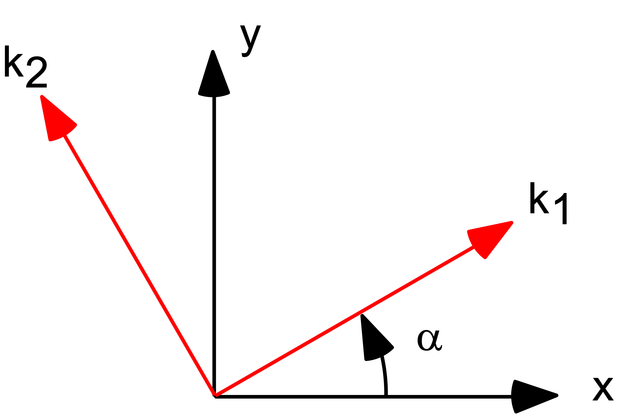
where \(k_1\) and \(k_2\) are the major and minor principal permeabilities respectively.
When the principal permeability directions are rotated by angle \(\alpha\) from the coordinate axes, the full conductivity tensor is computed using coordinate transformation:
\([K] = [R]^T [K_{principal}] [R]\)
where \([R]\) is the rotation matrix:
\([R] = \begin{bmatrix} \cos\alpha & \sin\alpha \\ -\sin\alpha & \cos\alpha \end{bmatrix}\)
This transformation yields the complete anisotropic conductivity tensor:
\([K] = \begin{bmatrix} k_1 \cos^2\alpha + k_2 \sin^2\alpha & (k_1 - k_2) \cos\alpha \sin\alpha \\ (k_1 - k_2) \cos\alpha \sin\alpha & k_1 \sin^2\alpha + k_2 \cos^2\alpha \end{bmatrix}\)
where:
\(k_1\) = the major principal permeability (typically horizontal for sedimentary soils)
\(k_2\) = the minor principal permeability (typically vertical for layered soils)
\(\alpha\) = the angle in degrees from the positive x-axis to the major permeability direction
If \(\alpha=0\), the K tensor reduces to:
\([K] = \begin{bmatrix} k_1 & 0 \\ 0 & k_2 \end{bmatrix}\)
For isotropic materials (\(k_1 = k_2 = k\)), the tensor reduces to \([K] = k[I]\) regardless of the rotation angle. In other words:
\([K] = \begin{bmatrix} k & 0 \\ 0 & k \end{bmatrix}\)
The continuity equation for incompressible flow in porous media requires that:
\(\nabla \cdot \vec{v} = 0\)
Combining Darcy's law with the continuity equation yields the governing equation for steady-state saturated flow:
\(\nabla \cdot ([K] \nabla h) = 0\)
Expanding this equation for two-dimensional flow with the full anisotropic conductivity tensor yields:
\(\dfrac{\partial}{\partial x}\left(k_{xx} \dfrac{\partial h}{\partial x} + k_{xy} \dfrac{\partial h}{\partial y}\right) + \dfrac{\partial}{\partial y}\left(k_{xy} \dfrac{\partial h}{\partial x} + k_{yy} \dfrac{\partial h}{\partial y}\right) = 0\)
which expands to:
\(k_{xx} \dfrac{\partial^2 h}{\partial x^2} + 2k_{xy} \dfrac{\partial^2 h}{\partial x \partial y} + k_{yy} \dfrac{\partial^2 h}{\partial y^2} = 0\)
When the principal permeability directions align with the coordinate axes (i.e., \(\alpha = 0°\) or \(k_{xy} = 0\)), this simplifies to:
\(k_1 \dfrac{\partial^2 h}{\partial x^2} + k_2 \dfrac{\partial^2 h}{\partial y^2} = 0\)
where \(k_{xx} = k_1\) and \(k_{yy} = k_2\). This elliptic partial differential equation governs the hydraulic head distribution throughout the seepage domain and forms the foundation for the finite element formulation implemented in XSLOPE.
Transient Flow Conditions
For completeness, transient flow analysis would require the governing equation:
\(\nabla \cdot ([K] \nabla h) = S_s \dfrac{\partial h}{\partial t}\)
where \(S_s\) is the specific storage coefficient. Such analysis would enable modeling of reservoir drawdown, rainfall infiltration, and construction dewatering scenarios.
Note
Transient flow analysis is not currently implemented in XSLOPE. The current implementation focuses on steady-state seepage problems only.
Unsaturated Flow Formulation
Unsaturated flow analysis becomes necessary when analyzing slopes with significant vadose zones above the phreatic surface. XSLOPE models the relative conductivity function with a linear front method by default — a simplified but robust approach for partially saturated conditions — and optionally with the van Genuchten model (v11+) or the Gardner power form (v14+), selected per material through the unsat property (lf, vg, or gard). The van Genuchten and Gardner models share one pair of law-agnostic input columns, a and n, whose meaning follows the selected unsat model.
The governing equation for steady-state unsaturated flow is:
\(\nabla \cdot (k_r(\psi) [K] \nabla h) = 0\)
where \(k_r(\psi)\) is the relative conductivity that varies with pressure head \(\psi = h - z\).
Linear Front Method for Relative Conductivity
XSLOPE uses a linear front method to define the relative conductivity function, implemented through the kr_frontal function. This method uses a simple piecewise linear relationship:
\(k_r(\psi) = \begin{cases} 1.0 & \text{if } \psi \geq 0 \text{ (saturated zone)} \\ kr_0 + (1 - kr_0) \left[ \dfrac{\psi - h_0}{-h_0} \right] & \text{if } h_0 < \psi < 0 \text{ (transition zone)} \\ kr_0 & \text{if } \psi \leq h_0 \text{ (dry zone)} \end{cases}\)
where: - \(\psi = h - z\) is the pressure head (negative in unsaturated zone) - \(kr_0\) is the relative conductivity at the reference suction head \(h_0\) - \(h_0\) is the reference suction head (negative value, typically -1.0 to -10.0)
The front can be visualized as follows:

This linear front approach provides several advantages:
- Computational Efficiency: Simple linear relationship avoids complex exponential functions
- Numerical Stability: Smooth transitions between saturated and unsaturated zones
- Physical Reasonableness: Captures the essential reduction in conductivity above the phreatic surface
- Parameter Simplicity: Only two parameters (\(kr_0\) and \(h_0\)) needed per material
The iterative solution process adjusts the relative conductivity within each element based on the computed pressure head sampled at the element's Gauss integration points (a quadrature-weighted average of \(k_r(\psi)\) over the element), creating a spatially varying conductivity field that reflects the degree of saturation throughout the domain.
Why the linear front is the default. For slope-stability seepage the precise shape of the unsaturated conductivity curve has little influence on the results. Negative pore pressures (suction) above the phreatic surface are conservatively neglected in both the limit-equilibrium and finite-element stability analyses, so the unsaturated zone never enters the strength calculation. And because the seepage solve is steady-state, the pore pressures below the phreatic surface — the ones that actually drive stability — are largely insensitive to the unsaturated curve. The linear front captures the essential conductivity reduction above the water table while remaining numerically robust, which is why it is XSLOPE's recommended model. The van Genuchten option below is provided chiefly for compatibility (e.g. importing models from other software) and user preference, not because it changes stability results.
van Genuchten Model
The van Genuchten–Mualem function is the most widely used relative-conductivity model in unsaturated soil mechanics. It is selected per material by setting unsat = "vg" and supplying two parameters, \(\alpha\) (entered in the a column) and \(n\) (the n column):
\(S_e = \left[\,1 + (\alpha\,|\psi|)^{\,n}\,\right]^{-m}, \qquad m = 1 - \dfrac{1}{n}\)
\(k_r(\psi) = \begin{cases} 1.0 & \psi \geq 0 \\ S_e^{\,1/2}\left[\,1 - \left(1 - S_e^{\,1/m}\right)^{m}\,\right]^{2} & \psi < 0 \end{cases}\)
Because the seepage solve is steady-state, only \(\alpha\) and \(n\) are needed — the residual and saturated water contents affect storage, not the relative conductivity, and so are not required. The function is evaluated at the same Gauss points as the linear-front model and is lightly regularized with a relative-conductivity floor (\(k_{r,\min}\approx10^{-4}\)) so the steep wet-end of the curve stays numerically robust; because suction is neglected in stability, the floor does not affect the stability results.
Typical parameter values. The table below gives representative van Genuchten \(\alpha\) and \(n\) by USDA soil-texture class, after Carsel & Parrish (1988) — the standard reference dataset (the same source used by HYDRUS and most unsaturated-flow codes). Use them as starting estimates and adjust to site data.
| Soil texture | a = α (1/cm) |
n |
|---|---|---|
| Sand | 0.145 | 2.68 |
| Loamy sand | 0.124 | 2.28 |
| Sandy loam | 0.075 | 1.89 |
| Loam | 0.036 | 1.56 |
| Silt | 0.016 | 1.37 |
| Silt loam | 0.020 | 1.41 |
| Sandy clay loam | 0.059 | 1.48 |
| Clay loam | 0.019 | 1.31 |
| Silty clay loam | 0.010 | 1.23 |
| Sandy clay | 0.027 | 1.23 |
| Silty clay | 0.005 | 1.09 |
| Clay | 0.008 | 1.09 |
Units of α
The \(\alpha\) values above are in 1/cm (the units in which Carsel & Parrish are tabulated). XSLOPE is unit-agnostic — the length unit is whatever the rest of the model uses — so convert \(\alpha\) accordingly: for metres multiply by 100 (1/cm → 1/m); for feet multiply by 30.48. \(n\) is dimensionless. As a rule of thumb, larger \(\alpha\) and \(n\) mean a coarser, more freely-draining soil (sands), while small \(\alpha\) and \(n \to 1\) mean a fine, slowly-draining soil (clays).
Gardner Model
The Gardner (1958) power form is the third option, selected with unsat = "gard" and the same two a / n
columns:
\(k_r(\psi) = \begin{cases} 1.0 & \psi \geq 0 \\ \dfrac{1}{1 + a\,|\psi|^{\,n}} & \psi < 0 \end{cases}\)
It is included for compatibility: this is the legacy relative-conductivity option in SEEP/W and Slide, so models imported from those packages carry \(a\) and \(n\) in exactly this form. Note that this is the power form of Gardner's function, not the exponential form \(k_r = e^{\alpha\psi}\) that also carries his name — the two are different functions, and the \(a\)/\(n\) pair only makes sense for the power form.
Unlike van Genuchten, there is no \(m = 1 - 1/n\) coupling, so \(n\) is not required to exceed 1; both \(a\) and \(n\) need only be positive. Like the other two models it is evaluated at the element Gauss points and floored at \(k_{r,\min}\).
Boundary Conditions
Proper specification of boundary conditions is essential for obtaining physically meaningful solutions to the seepage problem. XSLOPE supports the two primary types of boundary conditions commonly encountered in groundwater flow problems.
Specified Head Boundary Conditions (Dirichlet)
Specified head boundary conditions prescribe the hydraulic head value along portions of the domain boundary:
\(h = h_0\) on \(\Gamma_h\)
These conditions are appropriate for boundaries where the hydraulic head is known or can be reasonably estimated. Common applications include:
Reservoir Boundaries: Where the seepage domain interfaces with bodies of standing water such as reservoirs, lakes, or retention ponds. The hydraulic head equals the water surface elevation.
Constant Head Sources: Boundaries representing infinite sources of water at known elevations, such as large rivers or maintained water levels in drainage systems.
Impermeable Boundaries at Depth: Deep boundaries where groundwater is assumed to be at hydrostatic equilibrium, with hydraulic head equal to the elevation of the boundary.
The mathematical implementation of specified head conditions in the finite element system involves direct substitution of known head values into the global system of equations. Nodes lying on specified head boundaries have their hydraulic head values prescribed directly, reducing the size of the system that must be solved.
Exit Face Boundary Conditions (Seepage Face)
Exit face boundary conditions represent boundaries where groundwater can freely discharge to the atmosphere, such as slope faces or excavation walls. These boundaries present a more complex mathematical condition because the location of the phreatic surface (where pressure head equals zero) is not known a priori.
On an exit face boundary, the boundary condition is:
\(\psi = 0\) (pressure head = 0) for nodes where seepage occurs (i.e, total head = elevation)
\(\dfrac{\partial h}{\partial n} = 0\) (no flow) for nodes above the seepage zone
The challenge lies in determining which nodes along the potential exit face actually experience seepage discharge versus those above the phreatic surface where no flow occurs. This requires an iterative solution process where the position of the phreatic surface is updated based on the computed hydraulic head distribution.
XSLOPE implements a robust algorithm for handling exit face conditions:
- Initial Assumption: All nodes on potential exit faces are assumed to be seepage nodes with \(\psi = 0\).
- Solution and Check: The system is solved and the resulting hydraulic heads are examined.
- Boundary Update: Nodes where the computed head would result in \(\psi > 0\) (tension) are converted to no-flow boundaries.
- Iteration: The process repeats until the seepage face configuration stabilizes.
This iterative approach ensures that the final solution satisfies the correct boundary conditions while accurately locating the phreatic surface.
For higher-order boundary elements (tri6, quad8, and quad9), XSLOPE applies the seepage-face active set on a boundary-edge basis rather than activating midside nodes independently. Corner nodes are still checked with the usual head/flow criteria, but a quadratic boundary side is only treated as an active seepage edge when both corner nodes and the midside node satisfy the active criterion. This prevents partially active quadratic edges, keeps the seepage transition at element corners, and improves compatibility between the higher-order head solution and the resulting flow net near exit-face corners.
Specified Flux Boundary Conditions (Neumann)
A specified-flux boundary prescribes the rate at which water crosses a boundary rather than the head on it. The typical use is rainfall infiltration or recharge applied to the ground surface, where the water table position is an output of the analysis and so cannot be imposed as a head.
On a flux boundary,
\(-k \dfrac{\partial h}{\partial n} = q\)
where \(q\) is the normal Darcy velocity (length/time), taken positive into the domain. Note that \(q\) is a flow per unit area of boundary, not a total discharge over the boundary segment; the two differ by the length of the segment.
The flux enters the finite element system as a boundary load rather than a prescribed value. Its consistent nodal loads are obtained by integrating the flux against the element shape functions along each boundary edge lying on the flux line,
\(f_i = \displaystyle\int_\Gamma N_i \, q \, ds\)
which for a straight edge of length \(L\) carrying a uniform \(q\) gives \(qL/2\) at each node of a
linear (tri3) edge, and \(qL/6\), \(qL/6\), \(2qL/3\) at the two corners and the midside node of a
quadratic (tri6, quad8, quad9) edge. Each set sums to \(qL\), so the total water entering
through the edge is exactly \(qL\) regardless of element order. Because a flux boundary is a
natural boundary condition, its nodes remain unknowns in the solve — unlike specified-head
nodes, which are eliminated.
Two consequences are worth noting:
A model with only flux boundaries is singular. The flux condition constrains the gradient of the head, not the head itself, so head is determined only up to an additive constant. At least one specified-head boundary or exit face must be present, and XSLOPE raises an error if none is.
A flux boundary can be over-specified. Nothing in the mathematics prevents a user from forcing in more water than the material can transmit away; the solver simply raises the pressure at that boundary until the flow balances, which produces positive pore pressure at the ground surface. Physically the surface would pond to a small depth and the excess would run off, so the true infiltration would be less than the value entered. XSLOPE does not model that runoff, but it does warn when any flux node finishes with \(\psi > 0\) on an unconfined problem, which is the signal that the specified rate exceeds what the soil can accept and the result should not be trusted.
A flux boundary may overlap an exit face, which is the natural way to pose rain falling on a slope face that also seeps. The two conditions then interact node by node, according to whether that part of the face is currently saturated. Where the exit face is inactive — the face is unsaturated there, above the exit point — the node is still a free unknown, so the rain lands on it and infiltrates, and it counts toward the reported inflow. Where the exit face is active — saturated, held at atmospheric pressure — the head is prescribed and the applied load is discarded: rain falling on an already-draining face simply runs off, and is counted neither as inflow nor as outflow. As the water table rises, nodes cross from the first regime to the second, and the exit point migrates up the face.
The one posing XSLOPE will not resolve is an inflow onto a seepage face that exceeds what the
face can drain. Such a node has no steady answer under either condition — it floods while free,
and sheds the water while prescribed — so the iteration oscillates rather than converging. That is
the switching boundary condition described above, which XSLOPE does not model; the run will report
converged = False and warn about ponding rather than return a plausible-looking number.
Zero flux is the natural (do-nothing) condition and is already what an unspecified boundary carries, so a flux boundary only needs to be defined where the flux is non-zero.
Solution Process
Finite Element Formulation
The finite element implementation of the seepage problem in XSLOPE follows standard Galerkin procedures for elliptic partial differential equations. The weak form of the governing equation is derived by multiplying by a test function and integrating by parts:
\(\int_\Omega [K] \nabla N_i \cdot \nabla h \, d\Omega = \int_{\Gamma_q} N_i q \, d\Gamma\)
where \(N_i\) are the finite element shape functions, \(\Omega\) is the seepage domain, and \(\Gamma_q\) represents boundary segments where flow is prescribed.
The discretized system results in the global matrix equation:
\([K_{global}] \{h\} = \{Q\}\)
where \([K_{global}]\) is the global conductivity matrix, \(\{h\}\) is the vector of nodal hydraulic heads, and \(\{Q\}\) represents boundary flow conditions and source terms.
Element Types and Integration
XSLOPE supports multiple finite element types optimized for different accuracy and computational requirements:
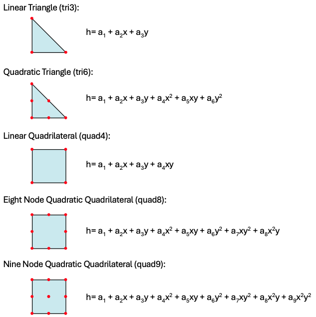
Linear Triangular Elements (TRI3): Provide computational efficiency and robust performance for most seepage problems. The constant hydraulic gradient within each element is well-suited for representing the smooth head distributions typical of groundwater flow.
Quadratic Triangular Elements (TRI6): Offer improved accuracy for problems with curved boundaries or complex head distributions. The quadratic head variation within elements better captures gradients near boundaries and interfaces.
Linear Quadrilateral Elements (QUAD4): Suitable for problems with regular geometric features where structured meshing is possible. Generally provide improved computational efficiency compared to triangular elements.
Higher-Order Quadrilateral Elements (QUAD8, QUAD9): Enable high-accuracy solutions for demanding applications, particularly those involving complex boundary geometries or strong material property contrasts.
The conductivity matrix for each element is computed using numerical integration:
\([K_e] = \int_{A_e} [B]^T [K] [B] \, dA\)
where \([B]\) is the strain-displacement matrix relating nodal heads to hydraulic gradients within the element.
Note
In most cases, linear triangles (tri3) are sufficiently accurate for seepage analysis.
Saturated vs Unsaturated Solution Algorithms
XSLOPE automatically determines whether to use saturated (confined) or unsaturated (unconfined) analysis based on the presence of exit face boundary conditions in the input. The solution approach differs significantly between these two cases:
Saturated Analysis (Linear Solution)
When no exit face boundary conditions are specified (i.e., no nodes with bc_type = 2), XSLOPE performs saturated analysis using the solve_confined function. This approach features:
- Linear System: Solves a single linear system \([K]\{h\} = \{Q\}\) where the conductivity matrix is constant
- Direct Solution: Uses sparse matrix factorization (
scipy.sparse.linalg.spsolve) - Computational Efficiency: Single solution step with guaranteed convergence
- Applicable When: The phreatic surface lies above or very close to the entire analysis domain
Unsaturated Analysis (Iterative Solution)
When exit face boundary conditions are present (i.e., any nodes with bc_type = 2), XSLOPE performs unsaturated analysis using the solve_unsaturated function. This iterative approach features:
- Nonlinear System: Requires iterative solution because conductivity varies with pressure head
-
Iterative Process:
1. Initialize hydraulic head distribution (usually from saturated solution)
2. Compute pressure head \(\psi = h - z\) at each element's Gauss integration points
3. Evaluate relative conductivity using the linear front method at each point and take the quadrature-weighted element average: \(k_r = kr_{frontal}(\psi, kr_0, h_0)\)
4. Assemble modified conductivity matrix: \([K_{modified}] = k_r [K]\)
5. Solve linear system with current conductivity matrix
6. Check convergence (see below)
7. Repeat steps 2-6 until convergence or maximum iterations reached -
Convergence Criteria: A hybrid test — all three conditions must hold simultaneously: 1. Head change: \(||h_{new} - h_{old}||_\infty <\) tolerance (scaled to domain height). A head-change test alone is not sufficient: how a given head tolerance maps to mass-balance error varies from problem to problem, so a tolerance that gives good flow closure on one model can leave a percent-level imbalance on another. 2. Flow closure: the unsigned nodal flow residual at free nodes, evaluated with the conductivity matrix rebuilt from the current (unrelaxed) heads, must drop below
closure_tol(default 0.1%) of the inflow. This measures the remaining nonlinear (k_r) lag directly in flow units, so the reported flowrate balances toclosure_tolon every problem regardless of the head tolerance — the converged discharge is tolerance-independent. 3. Exit-face stability: the seepage-face active set must be unchanged from the previous iteration (the flowrate is not meaningful while exit nodes are still switching). - Exit Face Handling: Iteratively determines which nodes experience seepage discharge vs. no-flow conditions
- Higher-Order Exit Faces: For
tri6,quad8, andquad9meshes, seepage activity is updated edge-by-edge so a quadratic exit-face side is either fully active or fully inactive - Computational Cost: Significantly higher than saturated analysis due to nonlinear iterations
Solution Algorithm Selection
The run_seepage_analysis function automatically selects the appropriate solution method:
# Check if this is an unconfined (unsaturated) problem based on exit face BCs
is_unconfined = np.any(bc_type == 2)

if is_unconfined:
    # Use iterative unsaturated solver
    head, A, q, total_flow = solve_unsaturated(...)
else:
    # Use direct saturated solver
    head, A, q, total_flow = solve_confined(...)
This automatic selection ensures that users get the most appropriate solution method based on their problem setup without manual intervention.
Integration with Excel Input Templates
A seepage analysis in XSLOPE uses the profile line data in the Excel input template to define the problem geometry. In addition, hydraulic properties input as part of the materials table and there is also a dedicated tab (sheet) for seepage boundary conditions.
Material Properties Definition
Seepage analysis in XSLOPE leverages the existing material property framework established for limit equilibrium analysis, extending it to include the hydraulic parameters needed for groundwater flow calculations. The material properties are defined in the Excel input template on the "mat" (materials) worksheet, where each soil layer includes both mechanical and hydraulic property definitions.
The hydraulic properties for each material include:
k1 (Major Principal Permeability): The hydraulic conductivity in the direction of maximum permeability, typically corresponding to the horizontal direction in sedimentary deposits or the direction parallel to bedding planes. Units are typically m/s, ft/s, cm/s, or equivalent.
k2 (Minor Principal Permeability): The hydraulic conductivity in the direction of minimum permeability, often the vertical direction in layered soils. For isotropic materials, k2 equals k1, while anisotropic materials exhibit k2 < k1.
alpha (Permeability Angle): The angle (in degrees) by which the principal permeability directions are rotated from the coordinate axes. A value of 0° indicates that k1 aligns with the x-axis (horizontal), while 90° indicates that k1 aligns with the y-axis (vertical).
kr0 (Relative Permeability at Reference Suction): For unsaturated analysis, this parameter defines the relative conductivity (k_rel = k_unsat/k_sat) at a reference pressure head h0. This parameter enables modeling of partially saturated hydraulic behavior above the phreatic surface.
h0 (Reference Suction Head): The reference pressure head (negative value representing suction) at which the relative conductivity kr0 is defined. Together with kr0, this parameter defines a simplified two-point approximation of the unsaturated conductivity function.
Boundary Conditions Specification
The seepage boundary conditions are defined in the "seep bc" worksheet of the Excel template, providing a structured approach for specifying the complex boundary conditions typical of slope seepage problems.
Specified Head Boundaries: Up to three separate specified head boundary conditions can be defined, each consisting of:
- Head Value: The hydraulic head to be maintained along the boundary (in length units consistent with the coordinate system)
- Coordinate Sequence: A series of (x,y) coordinate pairs that define the geometric extent of the specified head boundary
The system automatically interpolates the specified head value along the line segments connecting the coordinate points, enabling representation of complex boundary geometries while maintaining constant head conditions.
Exit Face Boundaries: A single exit face boundary is defined through a sequence of coordinate pairs representing the potential seepage discharge locations. The system automatically determines which portions of this boundary actually experience seepage discharge based on the computed hydraulic head distribution.
Seepage Solution Integration
For problems requiring seepage analysis coupled with either limit equilibrium or finite element slope stability calculations, XSLOPE provides seamless integration through pre-computed seepage solutions. This approach separates the computationally intensive seepage analysis from the slope stability analysis, enabling efficient parameter studies and optimization workflows. This process is described in more detail in the Seepage - Slope Stability Integration section.
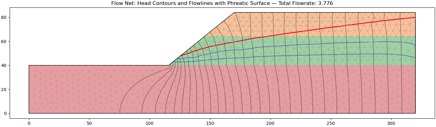
Flow Net Generation and Visualization
Beyond pore pressure calculation, XSLOPE provides comprehensive visualization capabilities for interpreting seepage analysis results through flow net generation and contour plotting.
Hydraulic Head Contours: Iso-head lines showing the spatial distribution of hydraulic head throughout the seepage domain. These contours are analogous to topographic contours and indicate the direction of groundwater flow (perpendicular to contour lines).
Flow Lines: Streamlines showing the paths followed by groundwater particles as they flow through the porous medium. These lines are generated by integrating the velocity field computed from the hydraulic head gradients using Darcy's law.
Phreatic Surface: The free groundwater surface where pore pressure equals zero (pressure head = 0). This surface represents the boundary between saturated and unsaturated zones and is critical for understanding groundwater behavior.
Velocity Vectors: Arrow plots showing the magnitude and direction of groundwater flow velocity at selected points throughout the domain. These vectors provide direct visualization of flow patterns and identify regions of high or low groundwater velocity.
The flow net generation algorithm computes streamlines by numerical integration of the flow velocity field:
\(\dfrac{dx}{dt} = -k_x \dfrac{\partial h}{\partial x}\)
\(\dfrac{dy}{dt} = -k_y \dfrac{\partial h}{\partial y}\)
where the velocity components are computed from the hydraulic head gradients using Darcy's law. The integration produces smooth streamlines that provide intuitive visualization of groundwater flow patterns and help identify potential seepage problems or areas requiring special attention in slope stability analysis.
Code Examples and Usage
Basic Seepage Analysis Workflow
The following example demonstrates the complete workflow for performing seepage analysis using XSLOPE's integrated mesh generation and solution capabilities:
from xslope.fileio import load_slope_data
from xslope.mesh import build_polygons, build_mesh_from_polygons
from xslope.seep import build_seep_data, run_seepage_analysis
from xslope.plot_seep import plot_seep_data, plot_seep_solution
import numpy as np

# Load slope geometry and material properties
slope_data = load_slope_data("inputs/slope/input_template_lface5.xlsx")

# Generate material zone polygons from profile lines
polygons = build_polygons(slope_data, debug=True)

# Create finite element mesh optimized for seep analysis
mesh = build_mesh_from_polygons(
    polygons=polygons,
    target_size=2.0,        # Element size in model units
    element_type='tri6',    # Quadratic triangles for accuracy
    debug=True
)

print(f"Generated mesh: {len(mesh['nodes'])} nodes, {len(mesh['elements'])} elements")

# Build seep analysis data structure
seep_data = build_seep_data(mesh, slope_data)

# Visualize mesh and boundary conditions
plot_seep_data(
    seep_data,
    show_nodes=True,
    show_bc=True,
    alpha=0.4
)

# Solve seep problem
solution = run_seepage_analysis(seep_data)

print(f"Seepage analysis complete!")
print(f"Head range: {np.min(solution['head']):.2f} to {np.max(solution['head']):.2f}")
if 'flowrate' in solution:
    print(f"Total flow rate: {solution['flowrate']:.6f}")

# Visualize results with flow net
plot_seep_solution(
    seep_data,
    solution,
    levels=20,              # Number of head contour levels
    base_mat=1,             # Material for flow line scaling
    fill_contours=True,     # Color-filled contours
    phreatic=True,          # Show phreatic surface
    mesh=True          # Overlay element edges
)
Import and Analysis of SEEP2D Files
For users with existing SEEP2D input files, XSLOPE provides direct import capabilities:
from xslope.seep import import_seep2d, run_seepage_analysis, print_seep_data_diagnostics
from xslope.plot_seep import plot_seep_data, plot_seep_solution

# Import SEEP2D format input file
seep_data = import_seep2d("inputs/seep/lface.s2d")

# Print diagnostic information about the imported data
print_seep_data_diagnostics(seep_data)

# Visualize imported mesh and boundary conditions
plot_seep_data(
    seep_data,
    show_nodes=False,
    show_bc=True,
    label_elements=False,
    label_nodes=False
)

# Run seep analysis
solution = run_seepage_analysis(seep_data)

# Plot results with customized visualization
plot_seep_solution(
    seep_data,
    solution,
    levels=25,
    base_mat=2,
    fill_contours=False,    # Line contours only
    phreatic=True,
    mesh=False,        # Clean visualization
    alpha=0.6
)
Advanced Analysis with Material Property Variations
This example demonstrates how to perform parametric studies by varying material properties:
from copy import deepcopy
import matplotlib.pyplot as plt

def parametric_seepage_study():
    """Perform parametric study of permeability effects on seep."""

    # Base case setup
    slope_data = load_slope_data("inputs/slope/input_template_lface5.xlsx")
    polygons = build_polygons(slope_data)
    mesh = build_mesh_from_polygons(polygons, target_size=1.5, element_type='tri6')

    # Define permeability ratios to study
    k_ratios = [0.1, 0.5, 1.0, 2.0, 5.0, 10.0]

    results = {}

    for k_ratio in k_ratios:
        # Modify material properties
        modified_data = deepcopy(slope_data)

        # Increase permeability of first material
        if modified_data['materials']:
            modified_data['materials'][0]['k1'] *= k_ratio
            modified_data['materials'][0]['k2'] *= k_ratio

        # Build seep data and solve
        seep_data = build_seep_data(mesh, modified_data)
        solution = run_seepage_analysis(seep_data)

        results[k_ratio] = {
            'head': solution['head'].copy(),
            'flowrate': solution.get('flowrate', 0.0)
        }

        print(f"k_ratio = {k_ratio}: Flowrate = {results[k_ratio]['flowrate']:.6f}")

    # Plot flowrate vs permeability ratio
    plt.figure(figsize=(10, 6))
    flowrates = [results[k]['flowrate'] for k in k_ratios]
    plt.semilogx(k_ratios, flowrates, 'o-', linewidth=2, markersize=8)
    plt.xlabel('Permeability Ratio')
    plt.ylabel('Total Flow Rate')
    plt.title('Seepage Flow Rate vs Material Permeability')
    plt.grid(True, alpha=0.3)
    plt.show()

    return results

# Run parametric study
parametric_results = parametric_seepage_study()
Export and Visualization of Results
from xslope.seep import export_seep_solution, save_seep_data_to_json
from xslope.mesh import export_mesh_to_json

def export_seepage_results():
    """Complete workflow with result export capabilities."""

    # Standard analysis workflow
    slope_data = load_slope_data("inputs/slope/input_template_lface5.xlsx")
    polygons = build_polygons(slope_data)
    mesh = build_mesh_from_polygons(polygons, target_size=2.0, element_type='tri6')
    seep_data = build_seep_data(mesh, slope_data)
    solution = run_seepage_analysis(seep_data)

    # Export mesh for reuse
    export_mesh_to_json(mesh, "outputs/seepage_mesh.json")
    print("Exported mesh to outputs/seepage_mesh.json")

    # Export seep solution for limit equilibrium analysis
    export_seep_solution(seep_data, solution, "outputs/seepage_solution.csv")
    print("Exported solution to outputs/seepage_solution.csv")

    # Save complete seep data structure
    save_seep_data_to_json(seep_data, "outputs/seep_data.json")
    print("Exported complete seep data to outputs/seep_data.json")

    # Plot 1: Mesh with boundary conditions
    plot_seep_data(seep_data, show_bc=True)

    # Plot 2: Solution with flow net
    plot_seep_solution(seep_data, solution, levels=25, phreatic=True,
                      fill_contours=True, mesh=True)

# Export complete analysis
export_seepage_results()
These examples demonstrate the full range of seepage analysis capabilities available in XSLOPE, from basic analysis workflows to advanced parametric studies and integration with limit equilibrium slope stability calculations. The modular design enables users to adapt these workflows to their specific analysis requirements while maintaining computational efficiency and solution accuracy.
References
Carsel, R.F., & Parrish, R.S. (1988). Developing joint probability distributions of soil water retention characteristics. Water Resources Research, 24(5), 755-769. https://doi.org/10.1029/WR024i005p00755
van Genuchten, M.Th. (1980). A closed-form equation for predicting the hydraulic conductivity of unsaturated soils. Soil Science Society of America Journal, 44(5), 892-898. https://doi.org/10.2136/sssaj1980.03615995004400050002x