Sensitivity

See Addressing a parameter and Discovering and specifying parameters for the parameter grammar sensitivity() and every other function on this page shares with Design and Back-Analysis.

Running a sweep

from xslope import load_slope_data
from xslope.sensitivity import sensitivity
from xslope.plot import plot_sensitivity

slope_data = load_slope_data("docs/lem/files/xslope_acads_simple.xlsx")

success, result = sensitivity(
    slope_data,
    param="mat:Soil:c",
    rel_range=0.5, n=9,          # ±50% about the base value, 9 points
    # values=[...],              # ...or give the values explicitly
    methods=("bishop", "spencer"),
    search=True,                 # re-search the critical surface per point
)
plot_sensitivity(result['df'], target_fs=1.2)

search=True is the default and the honest setting: the critical surface moves as parameters change, and re-solving a fixed surface silently understates sensitivity. search=False re-solves the stored surface (circles[0] or the non-circular polyline) instead — roughly fifty times faster, and correct when the question is "given this surface" (prescribed-surface benchmarks, for example).

The result is a tidy long-format DataFrame — one row per (value × method), with the unmodified model included as a flagged is_base row:

column	meaning
param	canonical reference, e.g. "mat:Soil:c"
value, rel	the swept value and value / base_value
is_base	this row is the unmodified model
method, fs	solver name and factor of safety
success, msg	per-point outcome — a failed point is a row, not an exception, so a sweep that breaks at value 7 of 9 still reports 1–6 (finding where things break is often the point)
Xo, Yo, R	the critical circle per point (searched sweeps), so a jump of the critical surface is visible in the data — plot_sensitivity draws jumped points open

plot_sensitivity draws one line per method with FS = 1 (and an optional target_fs) as guide lines, marks the unmodified model as a labelled base case entry in the legend — so the black square in the plot reads as base case (value, FS = …) rather than an unexplained point — and draws any point where the critical surface jumped as an open circle.

mode= selects the engine that evaluates each swept point (see Analysis modes: LEM, FEM, seepage). mode='lem' (the default) runs the limit-equilibrium methods and reports a factor of safety. mode='fem' runs a full SSRM solve at every point — the output is still a factor of safety, but each step is a complete finite-element analysis (expect minutes per step; run it in the background) and the model must carry a mesh in slope_data['mesh']. mode='seep' rebuilds and solves the seepage problem at every point and reports the total discharge q through the section (the same flow rate the seepage solver returns), and likewise needs a mesh. The result's value column stays fs for a consistent schema; result['output'] ('FS' or 'q') and result['output_label'] say what it really is, so a discharge sweep is never mislabelled a factor of safety.

Sweeping anything else: modify=

For changes that are not a single stored scalar — geometry above all — pass a callable instead of a parameter reference. The callable receives a copy of the model and the swept value, and owns whatever consistency its edit requires (rebuilding the material polygons and ground surface after moving profile points, keeping reinforcement anchored to a moved face):

import math
from shapely.geometry import Polygon
from xslope.fileio import build_ground_surface_from_polygons
from xslope.mesh import build_polygons

def set_slope_angle(sd, beta_deg):
    """Rotate the slope face about the toe to beta_deg, then rebuild the
    polygon geometry (slice weights come from the polygons, not the raw
    profile lines — see the Slope Design page for this pattern)."""
    prof = sd['profile_lines'][0]['coords']
    x_toe, y_toe = prof[1]
    _, y_top = prof[2]
    prof[2] = (x_toe + (y_top - y_toe) / math.tan(math.radians(beta_deg)), y_top)
    polys = [{'polygon': Polygon(p['coords']), 'mat_id': p['mat_id']}
             for p in build_polygons(slope_data={'profile_lines': sd['profile_lines'],
                                                 'max_depth': sd.get('max_depth')})]
    sd['polygons'] = polys
    sd['ground_surface'], sd['domain_polygon'] = build_ground_surface_from_polygons(polys)
    return sd

success, result = sensitivity(slope_data, modify=set_slope_angle,
                              label="slope angle (deg)",
                              values=[20, 22.5, 25, 27.5, 30],
                              methods=("bishop",))

Built-in references and modify= callables are one code path — every param reference resolves internally to exactly the setter signature modify= accepts — and the engine validates the modified model at every point (polygon validity, ground surface present) precisely because setters may be user-written: a broken edit becomes a success=False row naming what broke, never a silently inconsistent answer.

Sensitivity plots

A sweep across several parameters feeds a family of views. Which one to read depends on the question: which parameter matters most (tornado, scaled bars), how the answer moves across the range (spider), or where the uncertainty comes from (variance Pareto, Monte Carlo rank). Each is a function in xslope.plot; all are reachable from the Studio Parametric dialog's plot-type selector and from the assistant's parametric_sweep call. The tornado — the most common — is covered in its own section below.

Tornado diagrams

To compare several parameters at once, tornado() evaluates each at its low and high bound (two solves per parameter plus one shared base case) and plot_tornado draws the Duncan-style summary — horizontal bars of the FS swing, sorted so the parameter that matters most sits on top:

from xslope.sensitivity import tornado
from xslope.plot import plot_tornado

success, result = tornado(
    slope_data,
    ["mat:Soil:c", "mat:Soil:phi", "mat:Soil:gamma"],
    rel_range=0.25,              # ±25% per parameter...
    # bounds={"mat:Soil:c": (2.0, 5.0)},   # ...or explicit bounds per ref
    method="bishop",
)
plot_tornado(result)

For the shipped ACADS sample (a weak c–φ soil), the tornado ranks φ far ahead of c and γ — the ±25% φ band alone swings FS from 0.77 to 1.21 across FS = 1.

plot_tornado draws the base-case FS as a labelled vertical reference line and stacks the bars widest-on-top by default — the classic Duncan ordering that gives the diagram its name. Pass widest_on_top=False to invert the stack (widest at the bottom); the parameter is kept for programmatic callers, and Studio deliberately exposes no toggle for it.

When you have already run full per-parameter sweeps — a GUI that draws an FS-vs-value curve per parameter for click-through, for instance — tornado_from_sweeps() assembles the same diagram from those DataFrames with no extra solves, since plot_tornado reads each parameter's lowest- and highest-value FS:

from xslope.sensitivity import sensitivity, tornado_from_sweeps

sweeps = {ref: sensitivity(slope_data, param=ref, rel_range=0.25, n=5,
                           methods=("bishop",))[1]['df']
          for ref in ("mat:Soil:c", "mat:Soil:phi", "mat:Soil:gamma")}
result = tornado_from_sweeps(sweeps, method="bishop")   # {'df', 'base_fs', 'method'}
plot_tornado(result)

Scaled-sensitivity bars

scaled_sensitivity() estimates the local derivative \(\partial F/\partial p\) for each parameter with a central difference at ±1% (relative) about the base case, then reports it under three scalings so parameters with different units compare on one axis. plot_scaled_sensitivity() draws one vertical bar per parameter — height is the magnitude, color the sign (green: FS rises with the parameter; red: FS falls):

• elasticity (the default) — the dimensionless \(\dfrac{\partial F}{\partial p}\cdot\dfrac{p}{F}\), i.e. the percent change in FS per percent change in the parameter.
• per_1pct — the change in FS for a 1% change in the parameter.
• per_sigma — the change in FS for a one-σ change (offered only for parameters that carry a standard deviation).

from xslope.sensitivity import scaled_sensitivity
from xslope.plot import plot_scaled_sensitivity

ok, result = scaled_sensitivity(slope_data,
                                ["mat:Soil:c", "mat:Soil:phi", "mat:Soil:gamma"],
                                method="bishop")
plot_scaled_sensitivity(result, scaling="elasticity")

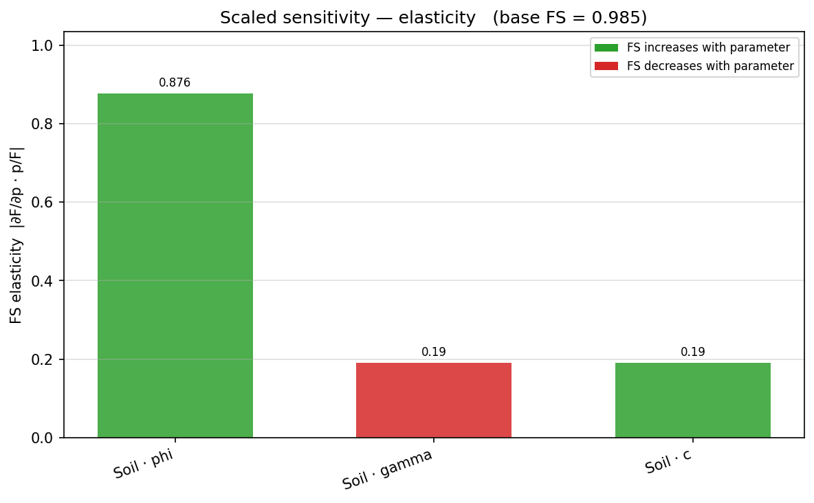
For the ACADS sample the friction angle dominates on the elasticity scaling — a percent change in φ moves FS several times more than a percent change in c or γ. The estimator (the central-difference derivative and each scaling) is documented in the scaled_sensitivity docstring.

Spider plot

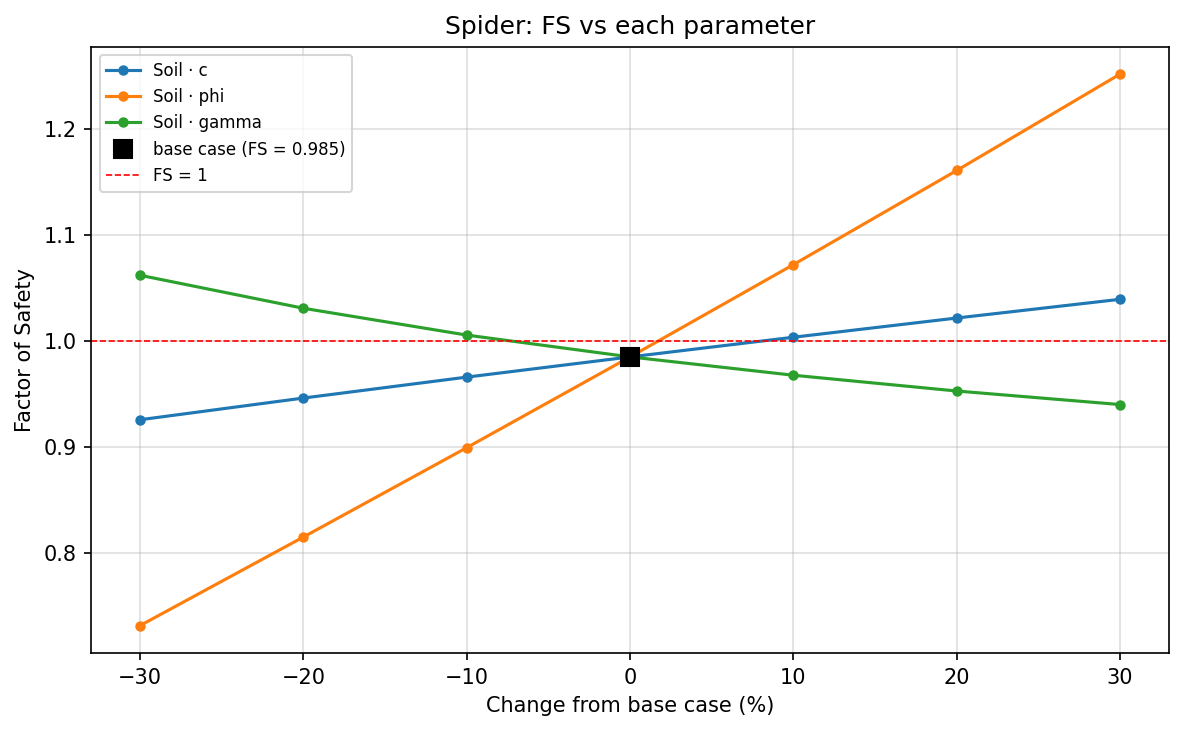
plot_spider() overlays every parameter's FS-vs-value curve on one normalized x-axis (percent change from the base value), with a black base-case marker at the origin and an FS = 1 guide. The steepness of each line is its sensitivity, and a curving line reveals nonlinearity a single tornado bar would hide. It reuses the per-parameter sweeps you already ran:

from xslope.sensitivity import sensitivity
from xslope.plot import plot_spider

sweeps = {ref: sensitivity(slope_data, param=ref, rel_range=0.3, n=7,
                           methods=("bishop",))[1]["df"]
          for ref in ("mat:Soil:c", "mat:Soil:phi", "mat:Soil:gamma")}
plot_spider(sweeps)

Variance-contribution Pareto

When the model carries standard deviations, variance_contribution() asks which uncertainties actually drive the scatter in FS. It reuses the Taylor-series reliability machinery — each parameter's variance term is \(\left(\dfrac{\partial F}{\partial p}\,\sigma_p\right)^2\), exactly the \((\Delta F/2)^2\) the TSPM already computes — normalizes each to a percent of \(\mathrm{Var}(F)\), and plot_variance_pareto() draws them descending with a cumulative line:

from xslope.sensitivity import variance_contribution
from xslope.plot import plot_variance_pareto

ok, result = variance_contribution(slope_data, method="bishop")
plot_variance_pareto(result)

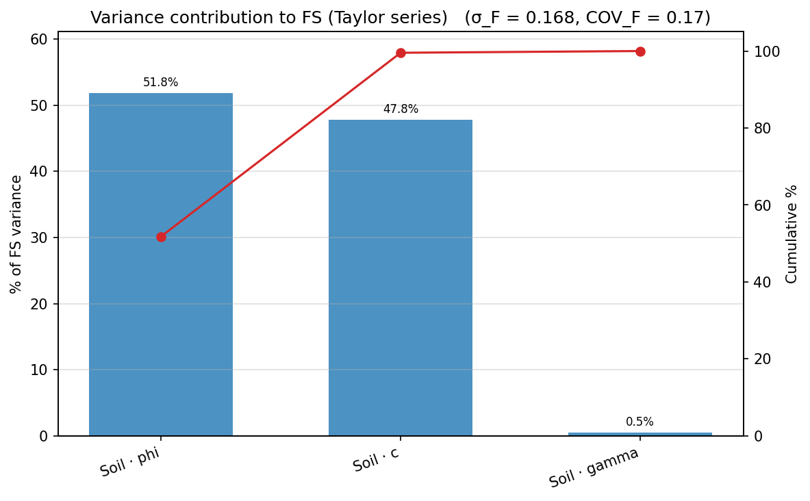
Note how this reorders the parameters versus the elasticity bars: c and φ contribute almost equally to \(\mathrm{Var}(F)\) even though φ has the larger elasticity, because c's standard deviation is a much larger fraction of its mean. A scaled bar answers how strong is the response; the Pareto answers how much does this parameter's uncertainty matter — the per-σ scaling above is the bridge between the two.

Monte Carlo rank correlation

mc_rank_correlation() runs a Monte Carlo reliability campaign and computes the Spearman rank correlation between each sampled input and the resulting FS. plot_mc_rank_correlation() draws them signed and sorted:

from xslope.sensitivity import mc_rank_correlation
from xslope.plot import plot_mc_rank_correlation

ok, result = mc_rank_correlation(slope_data, method="bishop", n_samples=10000)
plot_mc_rank_correlation(result)

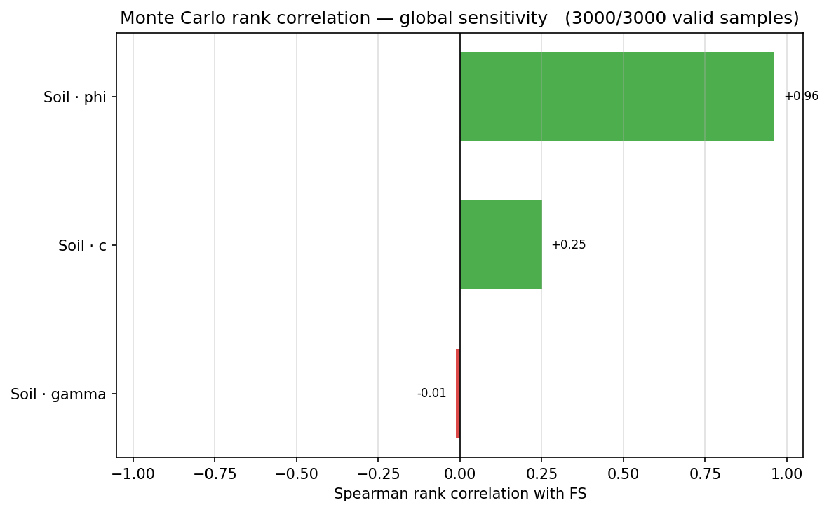
This is a global sensitivity measure: unlike the scaled bars — a derivative at the base case — it ranks parameters over the whole sampled distribution, so it captures a parameter's spread and any nonlinearity in its effect. The local and global measures can disagree, and the disagreement is itself informative; read the two together.

Worked sample

The sweep below reproduces the base case of the ACADS simple slope sample (xslope_acads_simple.xlsx, the same file used throughout these pages) and brackets it over ±50% of the cohesion, re-searching the critical surface at every point. The regression suite locks the end points: at c = 1.5 the critical circle has retreated toward the face (the surface-jump columns show the radius growing as cohesion falls), and at c = 4.5 the slope crosses FS = 1.

c (kPa)	Bishop FS
1.5 (−50%)	0.882
3.0 (base)	0.985
4.5 (+50%)	1.073

A geom:piezo:dy sweep on any of the water-table samples answers the most common geometry question — "how sensitive is this slope to the water table?" — without writing a setter: the reference shifts the piezometric line vertically by the swept delta.

For a published benchmark of the sweep itself, see verification problem VP40 — Perry (1993)'s power-curve sensitivity study, where the swept ΔFS matches Slide's published curves within about a percent at every range endpoint.