Morgenstern–Price Method
The Morgenstern–Price method (Morgenstern & Price, 1965) is a complete-equilibrium procedure: like Spencer's method it satisfies force equilibrium (horizontal and vertical) and moment equilibrium for the sliding mass, and it applies to both circular and non-circular surfaces. It is the most general of the limit-equilibrium methods in XSLOPE, and Spencer's method is a special case of it.
Relationship to Spencer's Method
Every slice has the same free body as in Spencer's method — refer to the Spencer slice geometry for the definition of every symbol (\(W\), \(N\), \(S\), the interslice resultant \(Z\) and its inclination \(\theta\), the external loads \(kW\), \(P/D\), \(T\), \(R\), \(V\), \(H\), and the angles \(\alpha\), \(\beta\), \(\theta_p\)):
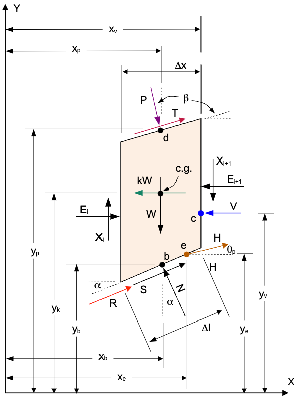
⚠ TODO (figures): redraw this force diagram in LibreOffice Draw — show the reinforcement force \(R\) at a general angle \(\psi\) at point \(r\) (not tangent to the base), and add the line load \(L\) at angle \(\delta\) at point \(f\) on the top of the slice.
The two methods differ in exactly one assumption — how the inclination of the interslice resultant is allowed to vary along the surface. Writing the interslice shear \(X\) and normal \(E\) at a slice boundary, the side-force inclination is \(\tan\theta = X/E\), and:
| Method | Interslice inclination | Unknowns |
|---|---|---|
| Spencer | constant: \(\tan\theta = \lambda\) everywhere | \(F,\ \lambda\) |
| Morgenstern–Price | varies: \(\tan\theta(x) = \lambda\, f(x)\) | \(F,\ \lambda\) |
Here \(f(x)\) is a prescribed, dimensionless interslice force function and \(\lambda\) is a single scalar that scales it. Setting \(f(x) = 1\) recovers a constant inclination — Morgenstern–Price with \(f(x)=1\) is identical to Spencer's method. XSLOPE uses this as the primary verification of the implementation: run with \(f(x)=1\), the factor of safety and \(\lambda\) reproduce Spencer's \(F\) and \(\theta\) to roughly \(10^{-10}\).
The Interslice Force Function
XSLOPE provides two interslice force functions, selected with the f_type argument
(half_sine is the default):
- Constant,
f_type='constant': \(f(x) = 1\). Reduces to Spencer's method; used as the regression case. - Half-sine,
f_type='half_sine':
\(f(x) = \sin\!\left(\pi\,\dfrac{x - x_L}{x_R - x_L}\right)\)
where \(x_L\) and \(x_R\) are the left and right ends of the slip surface. The half-sine drives the interslice shear smoothly to zero at both ends of the surface, which is physically reasonable (no shear can be transmitted past the crest or the toe). This is the textbook default and matches the default used by GeoStudio SLOPE/W, so it is the most useful choice for comparison.
The computed factor of safety is famously insensitive to the choice of \(f(x)\); \(\lambda\), on the other hand, does depend on it (see Insensitivity to f(x) below).
Force Equilibrium — the Per-Slice March
For a trial factor of safety \(F\) and trial scale \(\lambda\), the per-boundary inclinations are fixed by the interslice assumption,
\(\theta_j = \arctan\!\big(\lambda\, f(x_j)\big), \qquad j = 0,1,\dots,n\)
evaluated at every slice boundary. With the inclinations known, the slices are marched left to right, solving on each slice the same \(2\times 2\) force-balance system used by the force-equilibrium methods — two equations (\(\sum F_x = 0\), \(\sum F_y = 0\)) in two unknowns, the base normal \(N_i\) and the right-hand interslice resultant \(Z_{i+1}\), given the left resultant \(Z_i\) carried over from the previous slice. The base shear enters through the mobilized strength
\(S_i = \dfrac{c'_i\,\Delta\ell_i + (N_i - u_i\,\Delta\ell_i)\tan\phi'_i}{F}\)
The march starts from \(Z_0 = 0\) (no force outside the first slice) and ends with a leftover interslice resultant \(Z_n\) at the downhill end. Global force equilibrium requires that this leftover vanish:
\(\text{force residual} = Z_n = 0\)
This is exactly the residual the Corps of Engineers and Lowe–Karafiath methods root-find on; the only difference is that those methods fix the \(\theta_j\) from geometry, whereas Morgenstern–Price chooses \((F,\lambda)\) to satisfy moment equilibrium as well.
Moment Equilibrium about the Origin
The second condition is overall moment equilibrium. XSLOPE sums moments for the whole sliding mass about the coordinate origin \((0,0)\). The origin is a fixed point that works identically for circular and non-circular surfaces — there is no reliance on a circle center, so the formulation is uniform across surface types.
The key simplification is that the interslice forces are internal: the force on the boundary between slices \(i\) and \(i+1\) acts on both adjacent slices with equal magnitude, the same line of action, and opposite sign. Summing moments over the entire mass, every interslice contribution cancels exactly, regardless of \(\lambda\) and regardless of where on the boundary the force acts. The overall moment equation therefore contains only the base normals \(N_i\), base shears \(S_i\), weights \(W_i\), and the external loads.
Taking counter-clockwise moments as positive, the moment about the origin of a force with global components \((F_x, F_y)\) acting at \((x,y)\) is \(M = x\,F_y - y\,F_x\). Summing the per-slice contributions:
| Force | Components \((F_x, F_y)\) | Acts at | Moment about origin |
|---|---|---|---|
| Weight \(W\) | \((0,\ -W)\) | \((x_c,\ y_{cg})\) | \(-W\,x_c\) |
| Base normal \(N\) (total) | \((-N\sin\alpha,\ N\cos\alpha)\) | \((x_c,\ y_{cb})\) | \(N\,(x_c\cos\alpha + y_{cb}\sin\alpha)\) |
| Base shear \(S\) | \((S\cos\alpha,\ S\sin\alpha)\) | \((x_c,\ y_{cb})\) | \(S\,(x_c\sin\alpha - y_{cb}\cos\alpha)\) |
| Surface load \(D\) | \((D\sin\beta,\ -D\cos\beta)\) | \((d_x,\ d_y)\) | \(-D\,(d_x\cos\beta + d_y\sin\beta)\) |
| Seismic \(kW\) | \((-kW,\ 0)\) | \((x_c,\ y_{cg})\) | \(kW\,y_{cg}\) |
| Tension-crack water \(V\) | \((-V,\ 0)\) | \((x_v,\ y_t)\) | \(V\,y_t\) |
| Reinforcement \(R\) | \((R\cos\psi,\ R\sin\psi)\) | \((x_r,\ y_r)\) | \(R\,(x_r\sin\psi - y_r\cos\psi)\) |
| Pile \(H\) | \((H\cos\theta_p,\ H\sin\theta_p)\) | \((x_h,\ y_h)\) | \(H\,(x_h\sin\theta_p - y_h\cos\theta_p)\) |
| Line load \(L\) | \((L\cos\delta,\ L\sin\delta)\) | \((x_f,\ y_f)\) | \(L\,(x_f\sin\delta - y_f\cos\delta)\) |
The reinforcement force angle is \(\psi = \alpha\) with \((x_r, y_r)\) at the base center for Dir = Tangent (flexible, the default), or the line's own inclination at the actual crossing point for Dir = Axial. The line load \(L\) acts at angle \(\delta\) (default \(-90°\), straight down) at point \(f\) on the top of the slice.
The total base reaction is split into the effective normal \(N'\) and the pore-water uplift \(U = u\,\Delta\ell\), both acting in the \((-\sin\alpha, \cos\alpha)\) direction, so the normal moment term is \((N' + u\,\Delta\ell)(x_c\cos\alpha + y_{cb}\sin\alpha)\). Because the base shear \(S_i\) carries the \(1/F\) factor, the moment sum is an equation in \(F\) for each trial \(\lambda\); its root is the moment factor of safety \(F_m(\lambda)\). The scale \(\lambda\) still enters this sum, but only indirectly through the \(N_i\): the per-slice vertical balance contains the net interslice shear \(X_{i+1} - X_i = \lambda\,(f_{i+1}E_{i+1} - f_i E_i)\), so changing \(\lambda\) redistributes the base normals and moves the moment sum.
Solving for F and λ
Define the two factor-of-safety curves obtained from the march at a fixed \(\lambda\):
- \(F_f(\lambda)\) — the \(F\) that drives the force residual \(Z_n\) to zero,
- \(F_m(\lambda)\) — the \(F\) that drives the moment residual to zero.
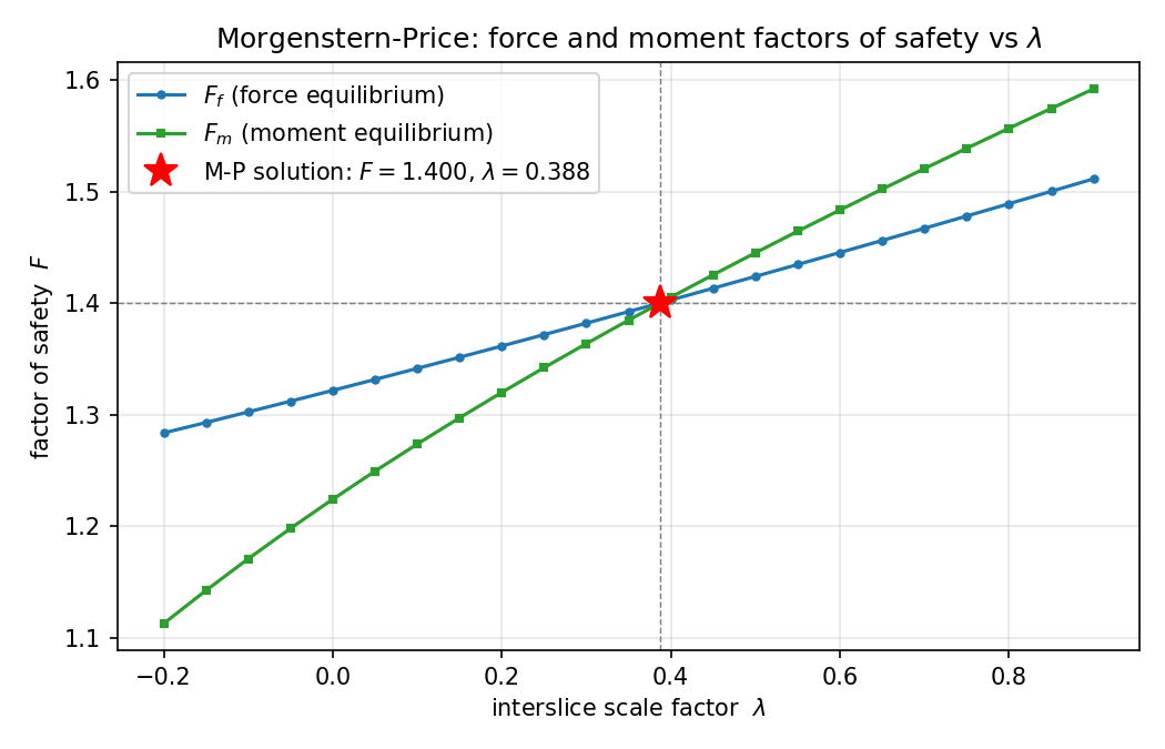
The Morgenstern–Price solution is the value of \(\lambda\) where the two curves meet, \(F_f(\lambda) = F_m(\lambda)\); the common value is the factor of safety. The two curves cross once and nearly linearly, as shown below for the Arai & Tagyo benchmark:
XSLOPE uses two cooperating solvers:
- Approach A (reference) — a robust two-curve crossing in the Fredlund–Krahn / GLE style: bracket \(\lambda\) and root-find \(g(\lambda) = F_f(\lambda) - F_m(\lambda)\) over \(\lambda \in [-1.5, 1.5]\), with an inner \(F\) root-find for each curve. This is transparent and produces the figure above directly, but does nested root-finds.
- Approach B (shipped) — a direct \(2\times 2\) Newton iteration that drives the
force and moment residuals to zero simultaneously in \((F, \lambda)\), seeded from
the Bishop factor of safety and \(\lambda = 0\), mirroring how
spencer()solves its \((F, \theta)\) system. It converges in a handful of evaluations and falls back to Approach A's bracketed crossing if it fails to converge.
Both solvers agree to roughly \(10^{-10}\) on every benchmark.
Admissibility guard. Because Morgenstern–Price optimizes \(\lambda\) to satisfy both equilibrium conditions, an unconstrained search can occasionally settle on a surface that balances only with partly tensile interslice forces — a non-physical mechanism that an automated critical-surface search would otherwise report as a spuriously low factor of safety. XSLOPE rejects a solution when more than 50% of the base normals are in tension or more than 30% of the interslice forces are tensile, returning failure so the search simply skips the surface (physical critical surfaces run at or below about 18% interslice tension).
Insensitivity to f(x)
A hallmark of the Morgenstern–Price method is that the factor of safety is nearly
independent of the assumed interslice force function. On a smooth circular surface
the spread between constant and half_sine is typically a few hundredths of a
percent. The spread is somewhat larger — around 1 to 1.5% — on non-circular
surfaces that run along a thin weak layer, where the sharp kinks in the slip
surface make the interslice force distribution matter more. This is expected
behavior, not a defect: it reflects genuine sensitivity of the mechanism, and even
there the factor of safety stays within about 1% of Spencer's value. The interslice
distribution itself (captured by \(\lambda\)) is more sensitive to \(f(x)\) than the
factor of safety is.
Line of Thrust
Once \(F\) and \(\lambda\) are found, the line of thrust — the line along which the interslice resultants \(Z\) act — is recovered exactly as in Spencer's method, except that the inclination now varies from boundary to boundary. Summing moments about the center of each slice base and solving for the right-hand thrust elevation,
\(y_{t,i+1} = y_b - \left[ \dfrac{M_o - Z_i \sin\theta_i \dfrac{\Delta x}{2} - Z_{i+1}\sin\theta_{i+1}\dfrac{\Delta x}{2} - Z_i\cos\theta_i\,(y_{t,i}-y_b)}{Z_{i+1}\cos\theta_{i+1}} \right]\)
with \(\theta_i = \arctan(\lambda f(x_i))\) at each boundary. Starting from the lower corner of the first slice and marching across, this traces the thrust line. With a constant inclination (\(f(x)=1\)) it reduces exactly to Spencer's expression.
Using the Method in XSLOPE
Morgenstern–Price is available as the method name mprice everywhere a method is
selected — in solve_selected(), the automated search algorithms, and
reliability analysis:
from xslope.solve import mprice

success, result = mprice(slice_df, f_type='half_sine')
if success:
    print(f"FS = {result['FS']:.3f}, lambda = {result['lambda']:.3f}")
The result dictionary mirrors Spencer's, with the addition of lambda and
f_type. Because the method solves a standard slice dataframe, it inherits
rapid drawdown and all external-load handling without any extra work.
References
- Morgenstern, N.R. & Price, V.E. (1965). The analysis of the stability of general slip surfaces. Géotechnique 15(1):79–93.
- Fredlund, D.G. & Krahn, J. (1977). Comparison of slope stability methods of analysis. Canadian Geotechnical Journal 14(3):429–439.