Running Analyses
Studio runs the same LEM, seepage, and FEM analyses as the xslope library, each
behind a run-options dialog. Long solves run on a background thread, so the window
stays responsive, with live output in the Log pane
and a Cancel button.
Pick the analysis type with the Mode selector, then click Run (its label follows the mode: Run LEM…, Run Seep…, Run FEM…).
Limit equilibrium (LEM)
In LEM mode, Run LEM… opens a dialog with:
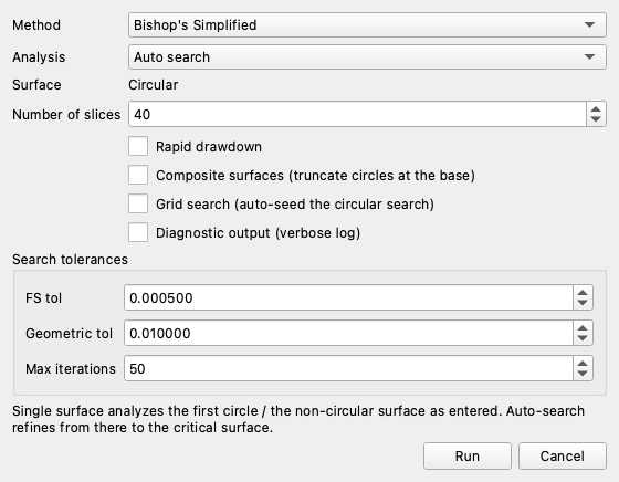
- Method — OMS, Bishop, Janbu, Corps of Engineers, Lowe & Karafiath, Spencer, or Morgenstern–Price.
- Analysis — single surface or automated search. (Probabilistic reliability analysis has its own toolbar button — see Reliability analysis below.)
- Surface — circular or non-circular (shown only when the file has both).
- Number of slices, the rapid drawdown flag, and a diagnostic toggle.
- Composite surfaces — lets a circle deeper than the bottom of the model be truncated at it and run along the base between the two crossings (see Composite Failure Surfaces). Off by default, and only available for circular surfaces. Turn it on when the base of the model is a real impenetrable boundary — bedrock, or a weak seam resting on it — because the critical mechanism there follows the base and no ordinary circle can reach it. Leave it off when the bottom of the model is simply how deep you chose to look.
- Grid search — seeds the circular search from an automatic grid-and-tangent sweep instead of (only) the circles sheet (see Grid Seeding). Off by default, available for circular auto-search. Turn it on to protect against the local-minimum trap of a single starting circle — a seed in the wrong family can converge 20% or more too high with no warning — or when you have no idea where the critical circle is (the circles sheet may even be empty). It reports the most critical surface anywhere in the model; leave it off to interrogate a specific mechanism with your own circles.
- Search tolerances (
fs_tol,tol,max_iter) — enabled for the search-driven analyses.
The result depends on the analysis type:
| Analysis | Result tabs |
|---|---|
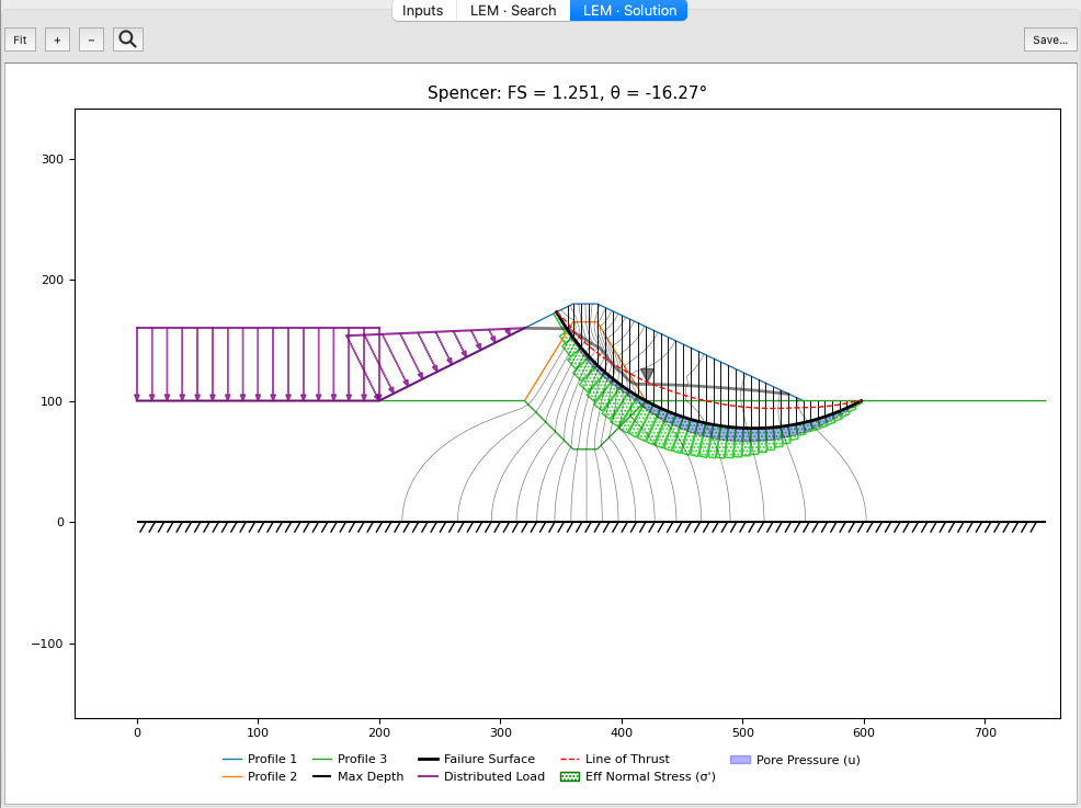
| Single surface | LEM · Solution — the surface with slices, base stresses, and thrust line. |
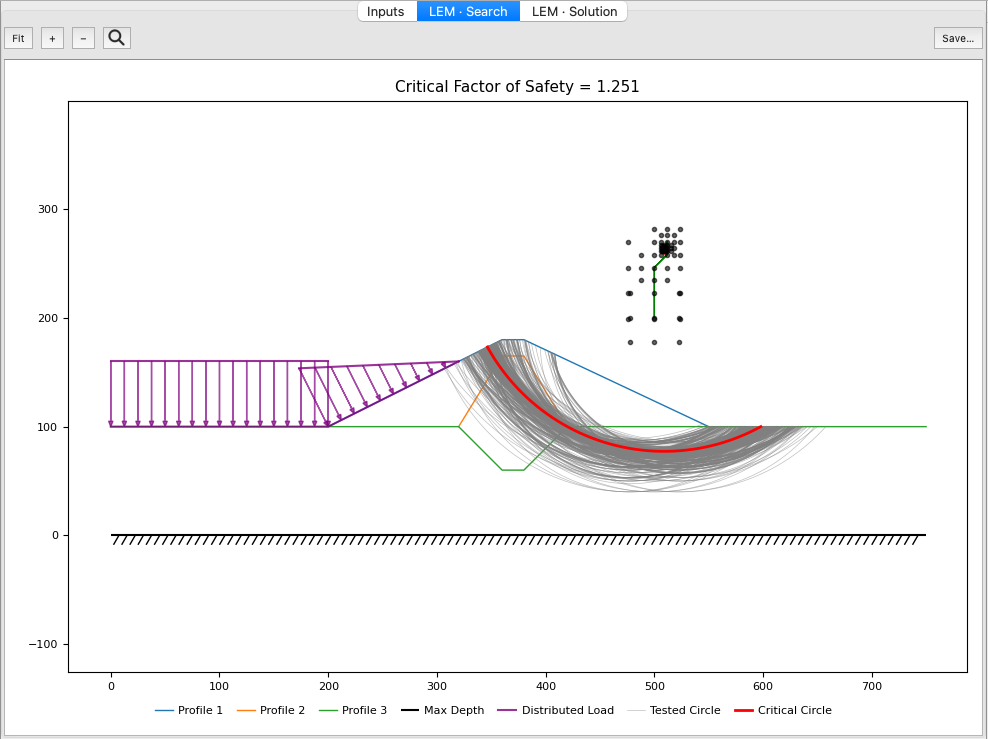
| Automated search | LEM · Search (all trial surfaces + critical + search path) and LEM · Solution (the critical surface). |
When the accepted solution carries admissibility defects — base tension on a cohesionless slice, interslice tension, or a line of thrust that leaves the slices — an amber strip across the top of the LEM · Solution view lists them, so an inadmissible FS is never mistaken for a clean success:
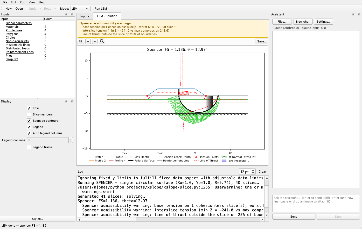
The warnings never change the factor of safety — they say the internal force distribution behind it is strained, and not all of them are equally alarming — see Interpreting the Admissibility Warnings. A clean solution shows no strip.
Both circular and non-circular surfaces are supported for single solves and searches. Search iteration progress streams to the Log pane, and a search can be cancelled from the status bar.
Parametric study
A second entry point sits beside Run — Parametric… — on both the Run menu
and the main toolbar, in all three modes (LEM, Seepage, FEM). It is available whenever
a model is open — in Seepage and FEM mode it additionally needs a built mesh, exactly like
Run — and is disabled while another analysis is running. Every version of it drives the
same sweep engine as the library — see
Parametric Studies for the engine, and the
/xslope skill for the scripted recipes.
One dialog covers three study modes, chosen by its Mode selector — Sensitivity,
Design, and Back-Analysis. In LEM three controls are shared by all of them:
Method (any of the seven LEM methods), Number of slices, and a Parameter picker —
a Material dropdown (each material plus a k_seismic (global) entry) and a Property
dropdown listing that material's option-aware sweepable fields (both drawn from the engine's
list_params). A Re-search the critical surface at each step checkbox applies throughout:
on by default — the honest setting, since the critical surface moves as the parameter changes
— and off re-solves the entered surface only (much faster, but right only for that prescribed
surface).
Sensitivity sweeps several parameters and visualizes how FS responds. A Plot type selector chooses the view — a tornado (the default), scaled-sensitivity bars (with a Scaling sub-choice: elasticity, per-1%, or per-σ), a spider plot, and — only when the model carries reliability standard deviations — a variance Pareto and a Monte Carlo rank correlation (with an MC samples count). The tornado, scaled, and spider plots sweep the parameters listed in the table; the variance and rank plots instead use every σ-carrying material automatically. The plots themselves are shown, with worked examples, on the Sensitivity engine page.
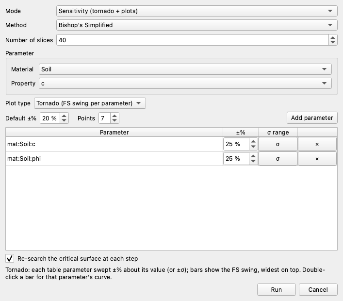
- A Default ±% and a Points count (points per parameter's FS-vs-value curve; the tornado uses only the curve's two endpoints, the spider draws the whole curve).
- Add parameter appends the currently picked material/property to the table. Each row shows the parameter reference, an editable ±% overriding the default for that row, a σ button, and a remove (✕) button.
- The σ preset swaps that row's ±% range for a ±one-standard-deviation range built from
the model's reliability
sigma_*columns — the same standard deviations the reliability analysis uses — so a sweep can mirror a reliability input band with one click. The button is disabled for a property that carries nosigma_*.
Design sweeps the one picked parameter toward a target FS:
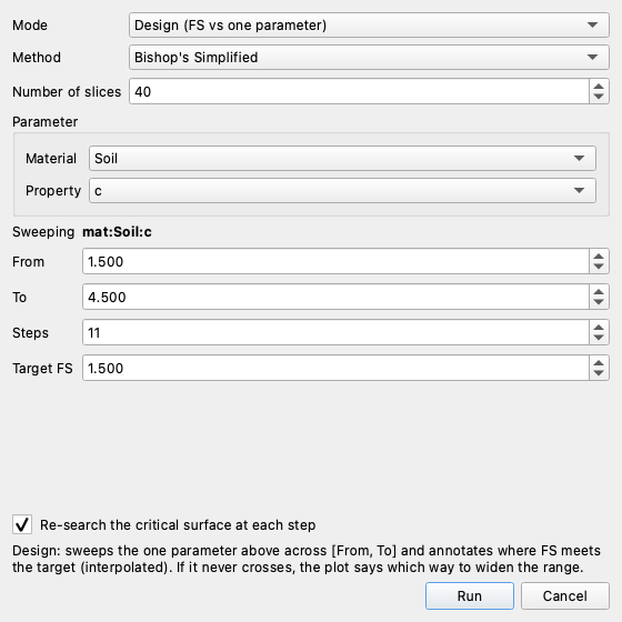
- From / To bound the swept value (seeded to ±50% of the current value the first time you pick a property), Steps sets the number of solves, and Target FS is the factor of safety to locate.
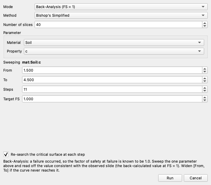
Back-Analysis is the same single-parameter sweep as Design, framed for a failure investigation: because a slide has occurred, the target defaults to FS = 1.0, and the result is read as the parameter value consistent with the observed failure (the back-calculated strength, most commonly). The controls are identical to Design.
Running and cancelling
Clicking Run launches the sweep on a background thread, so the window stays responsive.
The progress bar tracks each solve (done/total, with the current swept value echoed in the
status bar), the sweep log streams to the Log pane, and the
status-bar Cancel button aborts cooperatively — the in-flight solve finishes, then the
sweep stops and the app is left consistent, with no partial result stored.
Results
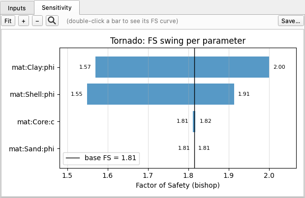
Sensitivity opens a Sensitivity tab with the selected plot. For the default tornado — one horizontal bar per parameter, widest on top, with the base-case FS drawn as a labelled vertical reference line:
On the tornado, double-click a bar to open a companion Sensitivity · Curve tab showing that parameter's full FS-vs-value curve (the base case marked, and any critical-surface jump drawn as an open circle):
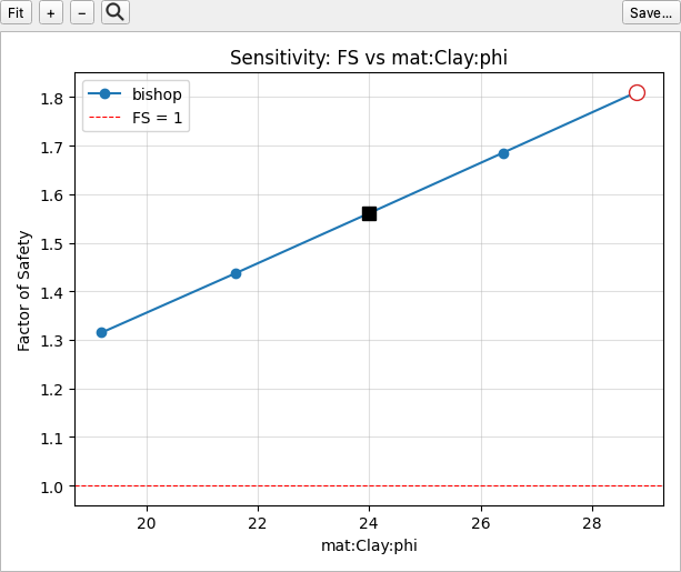
The other plot types render into the same Sensitivity tab — the scaled-sensitivity bars, the spider plot, the variance-contribution Pareto, and the Monte Carlo rank-correlation bars (the Sensitivity page shows each with a worked example). The double-click click-through is a tornado affordance; the other plots do not offer it.
Design opens a Design tab with the FS-vs-value curve, the FS = 1 and target-FS guide lines, and — when the target is bracketed — the interpolated crossing marked with a green diamond and annotated property = value for FS = target (a Back-Analysis run renders the same tab, with the target at FS = 1.0):
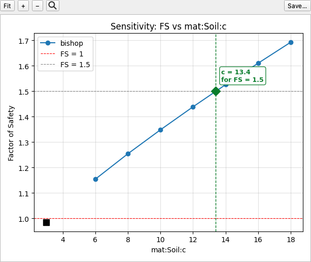
When the swept range never reaches the target, the result is honest about it: no crossing is drawn, and an amber note reports the FS span and which way to widen the range — the GUI face of the engine's never-extrapolate discipline:
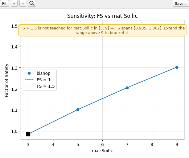
A sweep for each mode
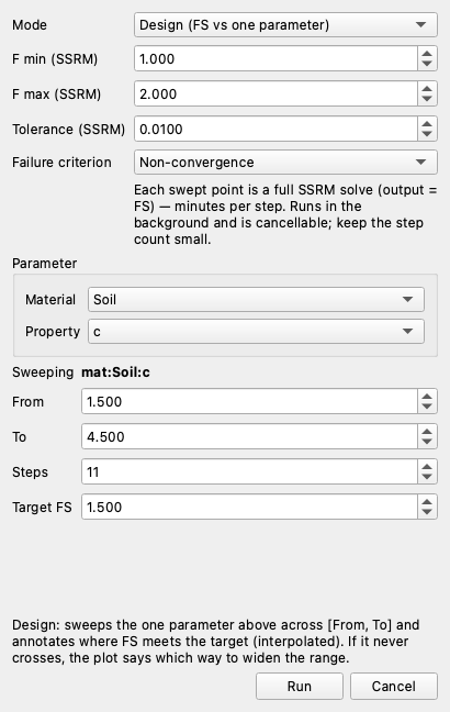
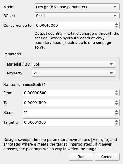
The Parametric dialog has a version for every mode. In LEM it sweeps the limit-equilibrium analyses (output: factor of safety). In FEM each swept point is a full SSRM solve (output: factor of safety) — expect minutes per step, so it runs in the background and is cancellable. In Seepage the output is the total discharge q through the section. FEM and seepage sweeps run on the mesh, so build one first. The variance Pareto and Monte Carlo rank plots reuse the LEM Taylor-series and Monte-Carlo reliability, so they are offered only for an LEM study that carries sigmas.
The dialog's solver rows follow the app mode: in FEM they become the SSRM knobs
(F_min / F_max, tolerance, failure criterion), and in Seepage they become the BC
set and convergence tolerance, with the design target a discharge q rather than an FS:
Reliability analysis
A Reliability… button sits beside Parametric… on the Run menu and the
toolbar — its probabilistic sibling. Where the Parametric study answers
deterministic what-ifs, Reliability turns the material standard deviations (the
s(·) columns of the mat sheet) into a reliability index β and a probability
of failure. It is available in LEM and FEM modes (not Seepage); the FEM run
needs a built mesh, like Run.
The dialog offers a Method selector with two engines:
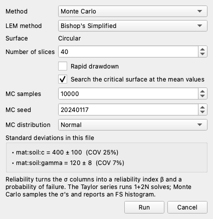
- Taylor series (TSPM) — the mean-value factor of safety plus a ±σ perturbation
of each uncertain parameter (
1 + 2Nsolves). Available in both modes; in FEM each factor of safety comes from an SSRM solve. - Monte Carlo — samples every uncertain parameter and evaluates the factor of safety of each realization on a fixed surface, reported as an FS histogram. Monte Carlo needs ~10⁴ solves, which is affordable with a limit-equilibrium solve but not with the finite-element SSRM, so it is disabled in FEM mode (a one-line note explains why, and FEM reliability stays on the Taylor series):
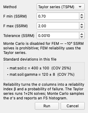
Below the engine controls, a read-only Standard deviations in this file summary
lists every s(·) column with its value, σ, and COV, so you can confirm what the run
will vary. LEM adds the solver method, surface, slice count, rapid-drawdown flag,
and a search the critical surface at the mean values toggle; Monte Carlo adds an
MC samples count, a seed (fixed by default, so the result is reproducible), and
a normal / lognormal distribution choice. FEM shows the SSRM F_min / F_max
bracket and a tight reliability tolerance. Settings are remembered for the session.
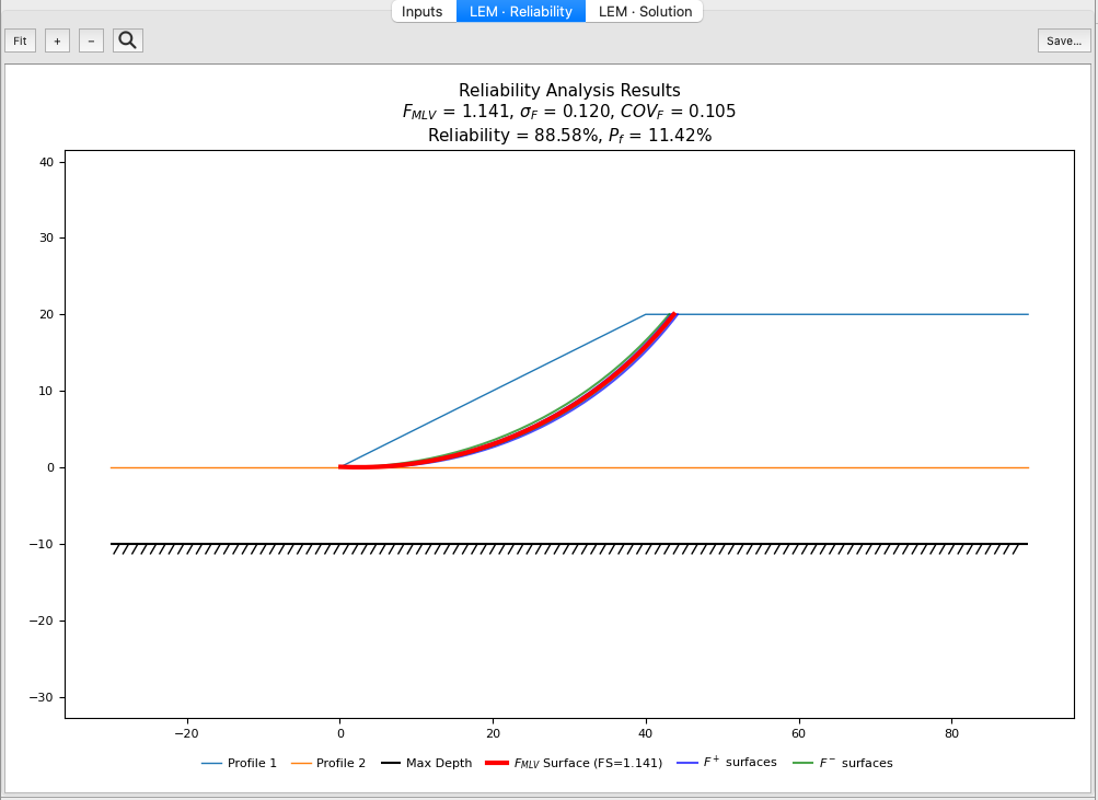
The run reports β, the probability of failure, and the mean / σ of the factor of safety in a summary, with the per-parameter table in the Log pane. The result view follows the engine:
| Engine | Result tab |
|---|---|
| Taylor series (LEM) | LEM · Reliability — the most-likely-value surface with the F⁺/F⁻ perturbation surfaces. |
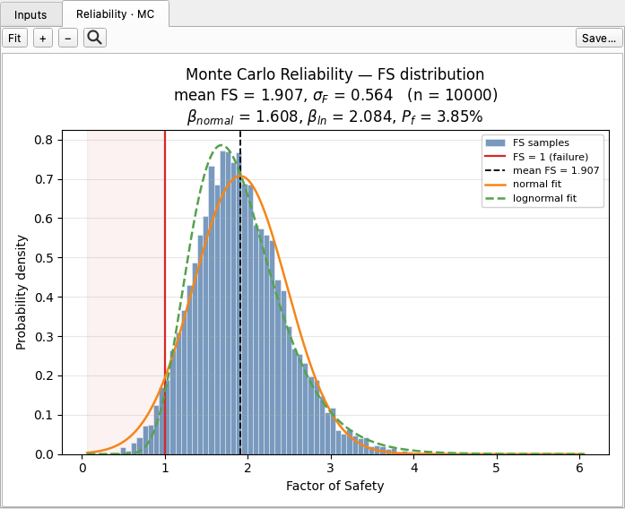
| Monte Carlo (LEM) | Reliability · MC — the FS histogram with the FS = 1 line, the mean, and fitted normal / lognormal overlays (a display-panel toggle). β in both conventions and the probability of failure are in the title. |
| Taylor series (FEM) | FEM · Results — the deformation at the most-likely values; β and the probability of failure are in the run summary. |
The engines are the same ones the library exposes — reliability (the front door),
reliability_taylor, reliability_mc, and reliability_fem; see
Reliability Analysis for the theory and worked examples.
Building a mesh
Seepage and FEM run on a finite-element mesh, which you build explicitly. In Seepage or FEM mode, Build Mesh opens a dialog with:
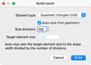
- Element type —
tri3,tri6,quad4,quad8, orquad9. - Target size — entered directly, or auto-sized as the slope width divided by a number of divisions.
- Refine near features — off by default. When checked, elements shrink near model
features (reinforcement/pile lines, crack tips, thin material zones) and grow back to
the target size away from them; the Refinement factor spinbox (default 3.0) sets
the local size to target size ÷ factor. Leaving it off builds exactly the mesh
earlier versions did. Refinement is detected automatically from the geometry — there
is nothing to place by hand. (Selecting individual feature classes is available in the
Python API via
refine_features; the dialog refines near all of them.)
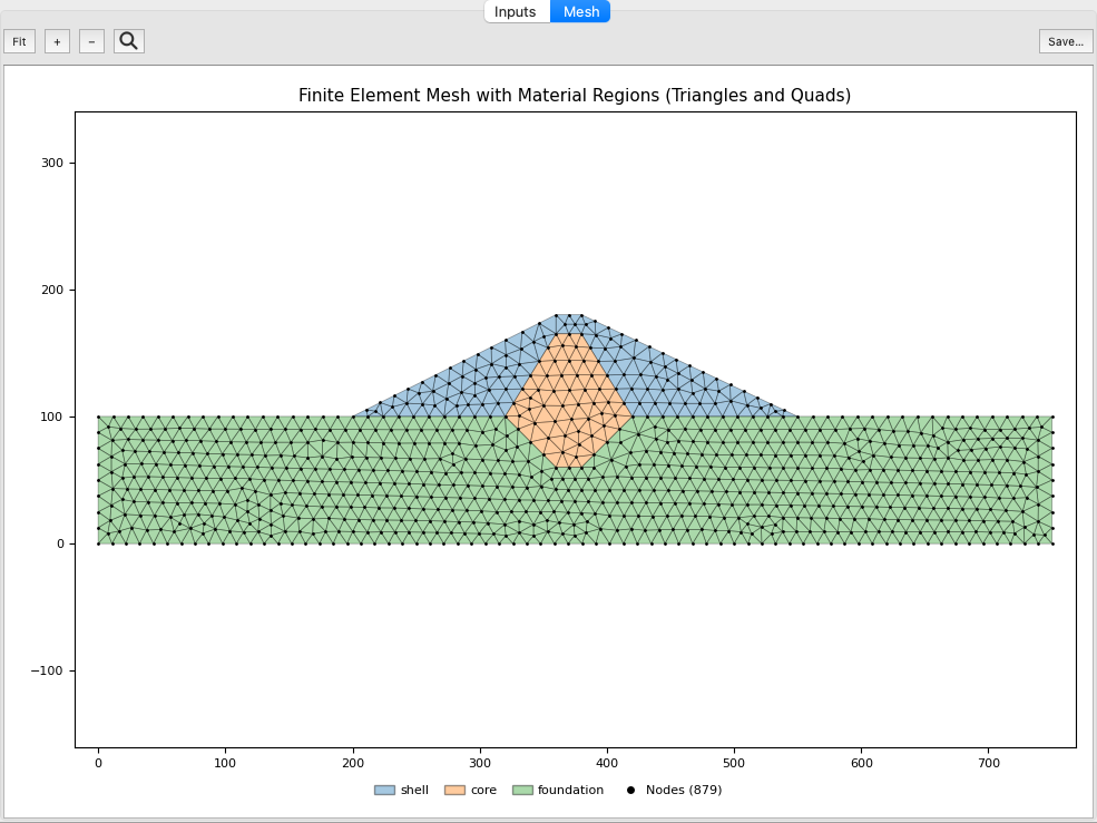
The mesh is built on a background thread (it includes reinforcement and pile
constraint lines, so it serves FEM too), shown in a Mesh tab, and written to a
{stem}_mesh.json sidecar. Seep/FEM Run stays disabled until a mesh exists; a
geometry edit that invalidates the mesh clears it and re-gates Run.
Meshing needs gmsh
Mesh generation uses gmsh, which is installed by the fem extra
(pip install "xslope[gui,fem]"). See Installation.
Seepage
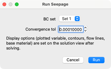
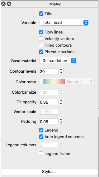
In Seepage mode, Run Seep… opens a dialog with just the solve parameters: the BC set (set 1, set 2, or both — the extra choices appear when the file defines a second set) and the convergence tolerance. Display choices — the plotted variable, contour levels, flow lines, vectors, fill, the phreatic surface — are not run options; they live on the Display panel of the solution view and re-render the cached solution without re-solving.
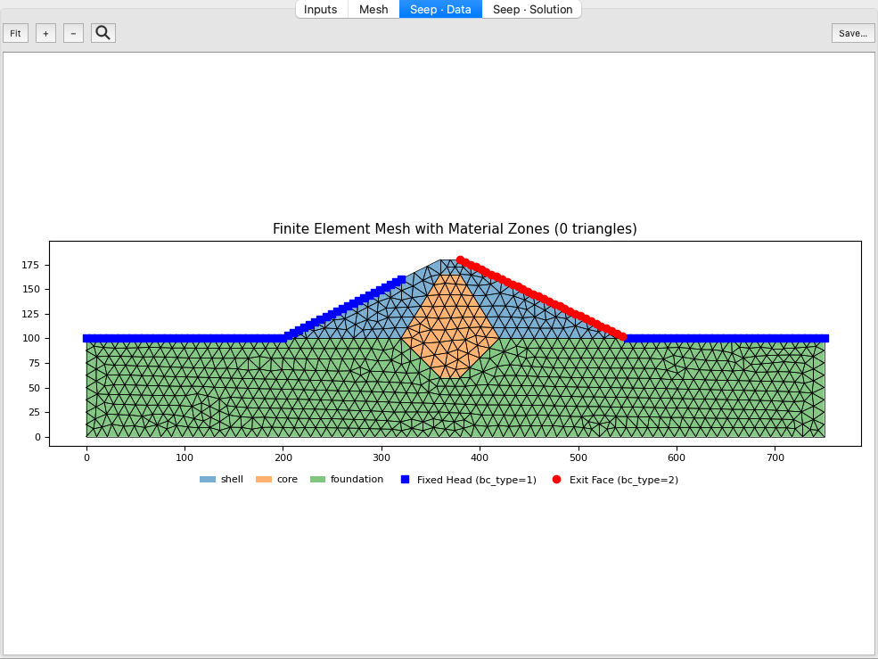
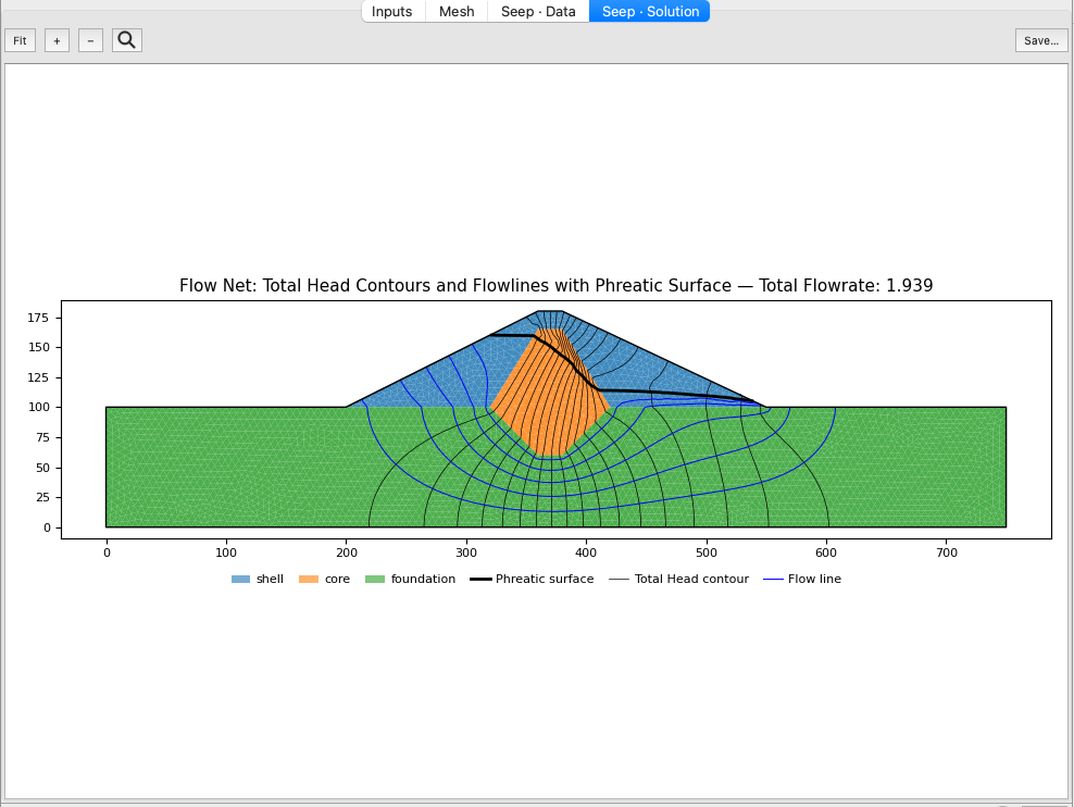
The run produces two tabs — Seep · Data (mesh + boundary conditions) and
Seep · Solution (the chosen variable, contours, phreatic surface, flow lines /
vectors) — and writes the solution to {stem}_seep.csv (_seep2.csv for BC 2).
The convergence trace streams to the Log pane. Each BC set keeps its own tab pair,
so rapid-drawdown problems show BC 1 and BC 2 together.
Finite element (FEM)
In FEM mode, Run FEM… offers a single trial or an SSRM run (the
Shear Strength Reduction Method), with F (or F_min/F_max), a tolerance, and
the failure criterion.
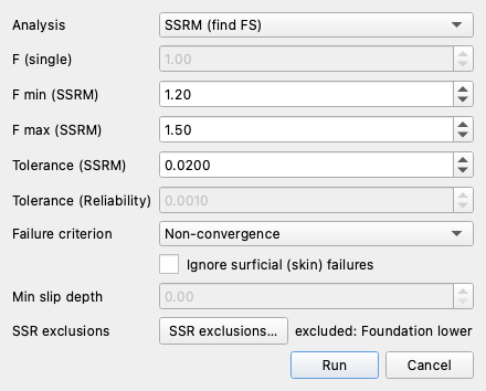
For an SSRM run, the SSR exclusions… button opens a checkbox picker — one row per material zone in the model, checked (included) by default:
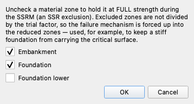
Unchecking a zone holds it at full strength through every trial factor instead of dividing its c and tan(φ) like the rest of the model — RS2's per-material Apply_SSR flag / SSR Exclusion Area. The mechanism is pushed up and out of an excluded zone, which is useful for keeping a non-participating zone (a stiff foundation, say) from carrying the failure, and for reproducing a vendor analysis that constrains the mechanism the same way — see SSR Exclusion Zones for the engineering rationale and a worked comparison against RS2. The button and the summary label next to it are gated to the SSRM analysis; the choice is a run option, not a model property, so it lives with the rest of the dialog's settings (remembered for the session to prefill the next run) rather than being saved into the input file.
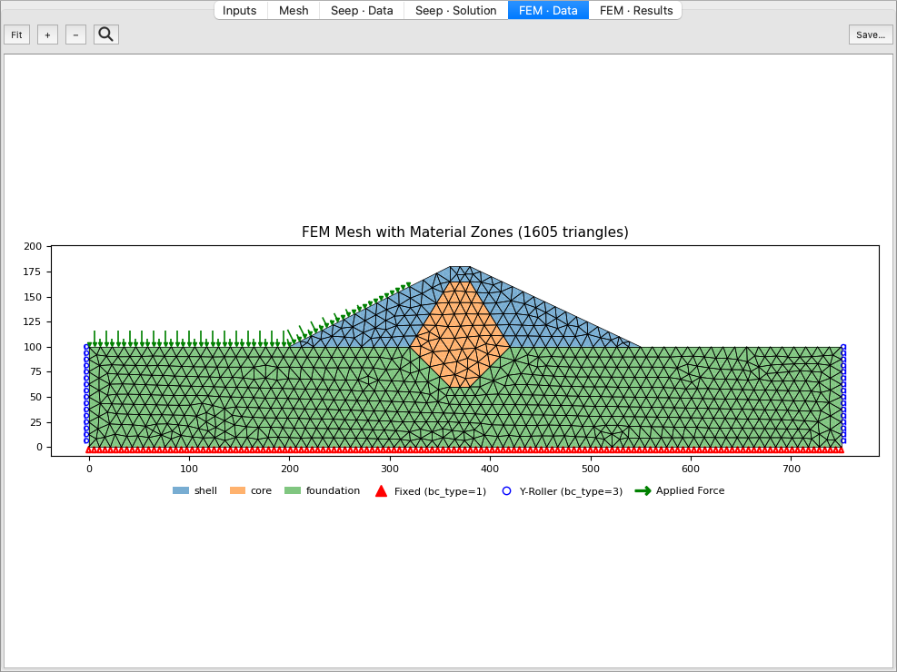
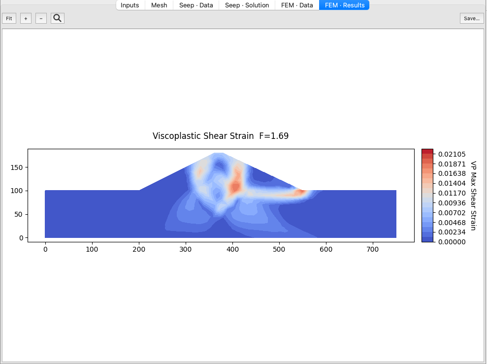
The run produces FEM · Data (mesh + boundary conditions + reinforcement) and FEM · Results (deformation, shear strain, displacement vectors). An SSRM run reports the factor of safety and can be cancelled mid-run. The solution is exported alongside the model so it can be restored on the next Open without re-solving.
Display options per view
Each result view has its own Display panel (in the left dock) exposing the options the underlying plot accepts — slice numbers and seep contours on the LEM solution; nodes / labels / padding on the mesh; variable, levels, vector scale, and flow-line toggles on the seep solution; plot type and deformation scale on FEM results; legend column layout on every view. Changing an option re-renders the cached result instantly — there's no re-solve. See The Display dock.
Exporting views: images and DXF
Every canvas has a Save… button that exports the current view:
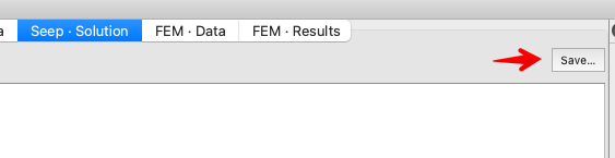
- Image — PNG, PDF, or SVG. PNG prompts for a DPI; vector formats don't. The figure is saved at its true inch size, so resolution is independent of the on-screen zoom.
- DXF (rendered view) — the drawn picture as a layered DXF, good for dropping into a CAD document. This is lossy as a re-import source; for that, use the structured geometry export below.
DXF import and export
Studio exchanges model geometry with CAD through DXF.
Export geometry — File → Export Geometry (DXF)… writes the structured, layered DXF: material zones on per-material layers, and profile lines, circles, reinforcement, distributed loads, and piezo lines on reserved feature layers. This is the clean companion the importer reads (distinct from the per-view rendered DXF above).
Import — File → Import DXF… opens a wizard that lists every layer in the drawing and lets you map each one to an input feature — material zone, profile line, piezo line, distributed load, reinforcement, failure circles, or ignore — with a material column for zones and profiles.
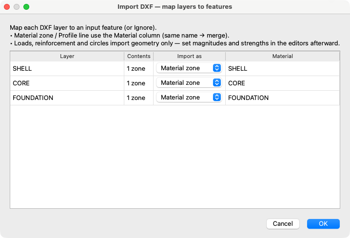
Defaults are seeded from xslope's own export layer names and the geometry kind, but you can override anything, so a DXF drawn in external CAD with arbitrary layer names maps just as well. Geometry populates the features; non-geometric properties (load magnitudes, reinforcement strengths, material properties, circle depth) come in as editable placeholders to fill in afterward. The import replaces the current project (you're prompted to discard first) and is left unsaved so you can complete it and Save As.
DXF layer conventions
The layer naming and entity conventions are shared with the library's
xslope.cad module — see DXF Import/Export for the full
layer table and format details.
DXF support needs ezdxf
Reading and writing DXF uses the ezdxf package (installed with the gui
extra). If it's missing, the import/export actions show an actionable install
message.
GeoStudio (SLOPE/W) import and export
Studio also exchanges whole models — not just geometry — with other slope-stability packages: GeoStudio SLOPE/W in both directions, and Rocscience Slide2 and RS2 as imports.
Import — File → Import GeoStudio (SLOPE/W)… reads a .gsz. Unlike DXF, there
is no mapping wizard to work through: a .gsz already knows what its geometry means, so
material zones, strengths, water conditions and the seismic coefficient all arrive
identified. The one prompt is which analysis to import, because a GeoStudio file
usually holds several over the same geometry — and they can differ in materials, not
just in slip surface, so the choice changes the model you get:
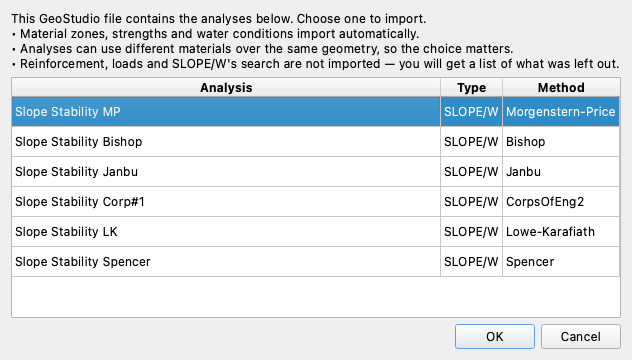
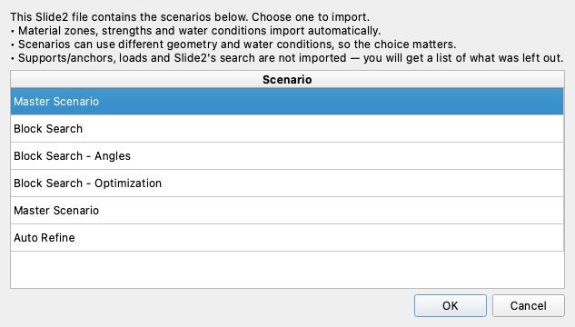
The other two vendor importers follow the same shape. File → Import Slide2… reads a
Rocscience Slide2 model (.sli / .slim / .slmd) and asks the same one question with a
scenario chooser, since a .slmd routinely bundles several scenarios over the same
geometry:
File → Import RS2 (.fez)… reads a Rocscience RS2 finite-element model. A .fez holds
exactly one model, so the only prompt is the file picker; geometry, materials and water
conditions import directly — including RS2's distributed and ponded-water loads, which are
converted to XSLOPE's perpendicular distributed loads — and whatever RS2 defines that cannot
cross (its SSR settings, joints, reinforcement, line loads and non-normal loads) comes back
in the post-import notes dialog. RS2's stability
result is an SSR field rather than a slip surface, so the import never carries a failure
surface — you define circles afterward.
Export — File → Export to GeoStudio (SLOPE/W)… writes the current model out as a
.gsz. It needs a polygon-based model (material zones), since a profile-line model has
no regions to map onto.
Both directions replace nothing silently: whatever cannot cross the format boundary — SLOPE/W's search definition, reinforcement, piles, loads, non-Mohr-Coulomb strengths — is listed in a notes dialog and in the Log pane, so you know exactly what to re-create by hand.
Units and what survives the trip
A .gsz carries no unit-system field, so XSLOPE infers it from the unit weight of
water and refuses to guess when it's neither metric nor imperial. See
GeoStudio Import/Export for the full mapping table, the
per-analysis materials wrinkle, and the limits of export.