Monte Carlo Reliability Analysis
The Monte Carlo method is a statistical technique that uses random sampling to estimate the probability of failure. It involves generating a large number of random samples for the uncertain parameters. Then we do the following steps:
- Generate N random samples for the uncertain parameters (e.g., soil unit weight, cohesion, angle of internal friction) based on their probability distributions.
- Combine random values for each uncertain parameter to create N "model instances". Each of these instances represents a unique combination of parameter values and is considered to be equally likely.
- Calculate the factor of safety for each model instance using a limit equilibrium method (e.g., Bishop's method, Janbu's method, or Spencer's method).
- Calculate the coefficient of variation of the factor of safety values obtained from the model instances.
While the Monte Carlo method is a powerful and flexible approach, it can be computationally expensive for slope stability problems as it requires a large number of model runs to obtain accurate results. The accuracy of the Monte Carlo method depends on the number of samples generated, and typically, thousands of model instances are needed to achieve a reliable estimate of the probability of failure.
Monte Carlo in xslope
The reliability_mc function runs a Monte Carlo campaign directly from the same
inputs as the Taylor series: the material most-likely values and the standard
deviations already in the mat sheet. Nothing new is required — "we just need a
number of runs, because we already have the standard deviations and the most-likely
values."
Sampling model. Each uncertain parameter is drawn independently from a
distribution whose mean is the material's base value (the MLV in the mat sheet)
and whose standard deviation is the matching s(·) column — s(g) for \(\gamma\),
s(c) for \(c\), s(f) for \(\phi\), s(c/p) for \(c_p\). The default distribution is
normal, the same interpretation the Taylor series places on those columns; a
distribution='lognormal' option draws lognormal samples matched to the same mean
and standard deviation. Every draw is truncated at its physical floor — a strength
or unit weight cannot go negative — which is the one modelling assumption beyond the
raw mean and sigma. That truncation is exactly the \(\phi \ge 0\) bound that governs
high-COV problems (see the VP34 worked example under
When to use Monte Carlo versus the Taylor series);
at ordinary COVs it never activates and Monte Carlo and the Taylor series
agree closely.
Number of runs and convergence. The default is 10,000 samples. The sample
mean and standard deviation of the factor of safety converge quickly (a few thousand
samples), but the empirical probability of failure — a count of the tail — converges
more slowly, so a small \(P_f\) needs more samples to resolve. Increase n_samples
until the reported \(P_f\) is stable to the precision you need.
Deterministic (seeded) sampling. The random-number generator is seeded from a
fixed constant (never the clock), so a given input file reproduces the same \(\beta\)
and \(P_f\) on every run — the results are regression-lockable. Pass a different
rng_seed to inspect sampling scatter.
Outputs. The function returns the sample mean factor of safety, its standard deviation \(\sigma_F\) and \(COV_F\), the reliability index in both conventions — a normal index \(\beta_N = (\bar F - 1)/\sigma_F\) and the lognormal \(\beta_{LN}\) from the sample moments (same formula as the Taylor series) — and the empirical probability of failure, the fraction of realizations with \(F < 1\), alongside the distribution-fitted normal and lognormal \(P_f\) for comparison. In XSLOPE Studio these samples are shown as an FS histogram with the FS = 1 line, the mean, and fitted normal / lognormal overlays — see Reliability analysis.
Limit-equilibrium only. Monte Carlo is available on the limit-equilibrium solvers only: a campaign of \(10^4\) factor-of-safety evaluations is affordable with a limit-equilibrium solve but not with the finite-element SSRM, so FEM reliability stays on the Taylor series (1 + 2N solves — see Reliability Analysis (FEM)).
Worked example: VP34 (Clarence Cannon Dam)
VP34 is the corpus case Monte Carlo was added for: Wolff & Harr (1987)'s Phase I
fill has \(\phi = 6.34° \pm 7.87°\), a coefficient of variation of 124%. The Taylor
series cannot evaluate \(F(\phi - \sigma)\) — MLV \(-\sigma\) is negative — and
reliability() declines the input; reliability_mc handles it by truncating the
negative draws at \(\phi = 0\), the same physical floor the published Monte Carlo
estimates apply (see When to use Monte Carlo versus the Taylor
series):
from xslope.fileio import load_slope_data
from xslope.advanced import reliability_mc
from xslope.plot import plot_reliability_histogram

slope_data = load_slope_data("vp034.xlsx")
success, result = reliability_mc(slope_data, "spencer", circular=False,
                                  search=False, n_samples=10000, num_slices=40)
plot_reliability_histogram(result)
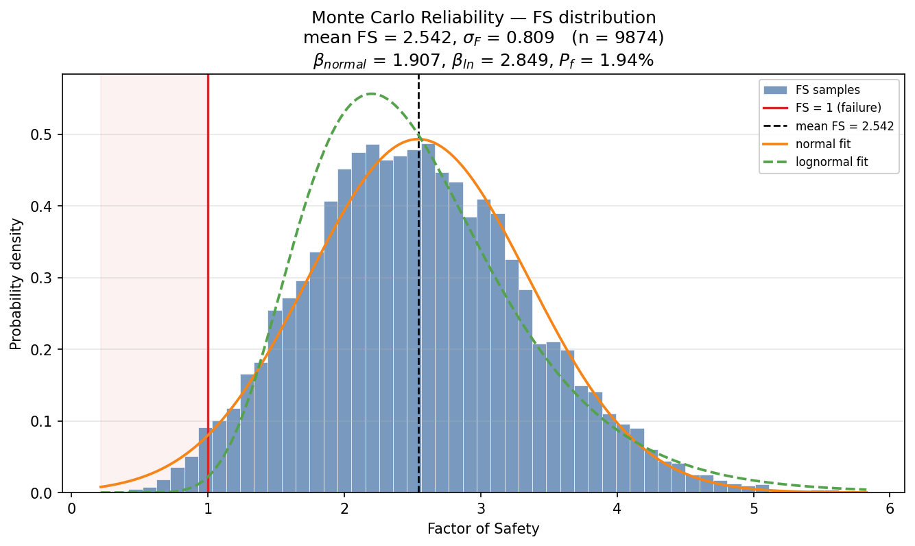
The distribution is strongly right-skewed, the signature of a large-COV input pushed through a nonlinear factor-of-safety response: mean FS = 2.542, \(\sigma_F\) = 0.809, and an empirical probability of failure of 1.94% (9,874 of the 10,000 draws converged to a valid Spencer solution; the rest are excluded rather than counted as failures). That lands inside the 0.36%–6.2% band spanned by the three published estimates for this problem — a case the Taylor series simply has no number for (see VP34 for the full comparison). This is the same plot XSLOPE Studio renders on the Reliability · MC result tab — see Reliability analysis.
Surface treatment
The slip surface is a decision variable, not a random variable — its geometry is therefore never randomized. Two treatments are meaningful:
- Fixed-surface Monte Carlo (the default). Every realization is evaluated on the
same surface: the prescribed surface when
search=False, or the most-likely-values critical surface whensearch=True(found once, then held fixed). This is the analogue of Slide2's Global Minimum probabilistic method, and it is what every published probabilistic benchmark did — Duncan's estimated LASH surface (VP29), Chowdhury & Xu's printed circles (VP28), Wolff & Harr's prescribed noncircular surface (VP34) — so it is the correct like-for-like basis for comparison. The honest caveat: a fixed-surface \(P_f\) understates the slope-system probability of failure, because for some sampled parameter sets the true critical surface lies elsewhere. - Per-realization minimum (a follow-up mode). The system-level analogue of Slide2's Overall Slope method re-evaluates, for each realization, the ensemble of candidate surfaces already found by the deterministic search and takes the minimum — not a fresh search per realization, which would be prohibitive. This mode is a documented follow-up and is not yet shipped; the fixed-surface campaign above is what the corpus comparisons use.
The Taylor-series side has the same distinction, already exercised in the corpus: on the Cannon Dam benchmark (VP35, Hassan & Wolff 1999) the surface of minimum reliability index is not the surface of minimum factor of safety, so a design screened on FS alone examines the wrong surface. Randomizing geometry is never the answer; searching on \(\beta\) (or on FS) is.