Transient Seepage in XSLOPE

Introduction

The seepage analysis described in the Overview solves for a single, time-independent hydraulic head field: it answers what does the flow field look like once it has settled? Many slope-stability problems, however, are governed by conditions that are still changing. A reservoir is drawn down over a few days; rain falls on a slope for a storm and then stops; a newly placed embankment sheds excess pore pressure over weeks. In each case the pore pressures that drive stability depend on when the slope is examined, and a steady-state solve cannot supply them.

Transient seepage adds the missing dimension. It solves the same finite-element groundwater flow problem repeatedly through time, marching a head field forward from an initial condition under boundary conditions that vary on a prescribed schedule, and storing the pore-pressure field at a series of saved times. Any one of those saved frames can then feed a limit-equilibrium or finite-element stability analysis in exactly the way a steady solution does, and two of them together drive a rapid-drawdown calculation.

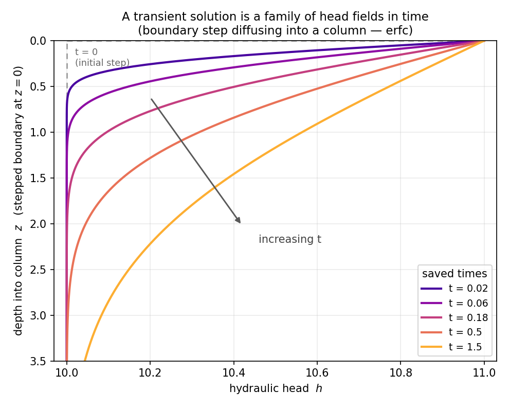
A transient solution is a family of head fields marched through time: here a sudden rise at the boundary spreads into a column, each curve one saved instant.

A seepage analysis becomes transient when the input file carries a filled-in tseep sheet (time series and run controls) and the materials carry storage properties. With no tseep sheet the analysis is steady-state and the results are bit-for-bit those of the Overview; the transient machinery is an additive path that leaves the steady solve untouched. This page describes the transient formulation, its storage physics, the time-stepping scheme, the boundary and initial conditions, the outputs, and the coupling to rapid drawdown.

Formulation

The steady seepage equation in the Overview balances the divergence of the Darcy flux against any distributed source, with no accumulation term:

\(\nabla \cdot (k_r(\psi)\,[K]\,\nabla h) = 0\)

This states that whatever flows into a control volume flows straight back out — the medium stores nothing. A transient problem relaxes exactly that assumption. When the head at a point changes, the water content of the surrounding soil changes with it, and the rate at which water is stored (or released) must be accounted for in the continuity balance. Reinstating the storage term gives the governing equation XSLOPE solves in a transient run:

\(\nabla \cdot (k_r(\psi)\,[K]\,\nabla h) + Q = S(\psi)\,\dfrac{\partial h}{\partial t}\)

where \(S(\psi)\) is the storage coefficient (specific storage where the soil is saturated, and the specific moisture capacity of the retention curve where it is not — see Storage properties), \(Q\) is any distributed source, and \(\partial h/\partial t\) is the local rate of change of hydraulic head. Setting \(S = 0\) (or holding \(h\) constant in time) recovers the steady equation above, so the transient solver is a strict generalization of the steady one.

Applying the standard Galerkin finite-element treatment used for the steady problem — multiply by a test function, integrate the conductivity term by parts — and discretizing the storage term with the same shape functions yields the semi-discrete matrix system

\([M]\,\dfrac{d\{h\}}{dt} + [K(\{h\})]\,\{h\} = \{Q\}\)

where \([K(\{h\})]\) is the (head-dependent, through \(k_r\)) global conductivity matrix from the steady solve and \([M]\) is the mass, or storage, matrix,

\(M_{ij} = \displaystyle\int_\Omega S(\psi)\,N_i\,N_j\,d\Omega\)

The conductivity matrix is assembled with the same batched, build-once machinery the steady solver uses — the saturated element stiffnesses and the \(k_r\) sampling operators are formed a single time and reused every step — and the storage matrix is assembled once in unit (density-one) form and rescaled by the current storage coefficient each iteration, exactly parallel to the way \(k_r\) rescales the stiffness. The time derivative is then integrated with the theta method described under Time stepping.

Storage properties

The storage coefficient \(S(\psi)\) is what makes a transient solve differ from a steady one, and its value depends on whether the soil is saturated. XSLOPE builds it from two per-material inputs carried on the mat sheet's Ss and Sy columns.

Specific storage \(S_s\)

Below the phreatic surface the soil is saturated and the storage that matters is specific storage \(S_s\) — the volume of water released from (or taken into) a unit volume of saturated soil per unit decline (or rise) in hydraulic head. It combines the compressibility of the soil skeleton and of the pore water, and it carries dimensions of inverse length (1/m or 1/ft, following the model's length unit). Representative magnitudes:

Material	\(S_s\) (1/m)
Plastic / soft clay	\(10^{-3}\) – \(10^{-2}\)
Stiff clay, dense silt	\(10^{-4}\) – \(10^{-3}\)
Sand	\(10^{-4}\) – \(10^{-3}\)
Dense sand and gravel	\(10^{-5}\) – \(10^{-4}\)
Fissured / jointed rock	\(10^{-6}\) – \(10^{-5}\)

\(S_s\) is required for every material in a transient run, because even a fully saturated, always-confined transient problem stores water through skeletal and fluid compressibility alone.

Specific yield \(S_y\)

Above the phreatic surface the dominant storage mechanism is not compressibility but drainage — water draining out of, or filling into, the pore space as the water table moves. This is governed by specific yield \(S_y\), the drainable porosity — a dimensionless quantity, always well below the total porosity because some water is retained against gravity. Representative ranges:

Material	\(S_y\) (–)
Clean sand and gravel	0.15 – 0.35
Fine sand	0.10 – 0.28
Silt	0.03 – 0.19
Clay	0.01 – 0.05

The finer the soil, the more of its pore water is held by capillarity and the lower its \(S_y\) — note the contrast with \(S_s\), which rises for softer, finer materials. For van Genuchten materials \(S_y\) doubles as the drainable water content \(\theta_s - \theta_r\), so a retention-curve fit is the better source when one exists. \(S_y\) enters the storage coefficient only through the unsaturated model, so it is needed only on unconfined (exit-face) transient problems; an always-saturated confined transient problem may leave it blank.

The specific moisture capacity \(C(\psi)\)

XSLOPE evaluates \(S(\psi)\) per element at the same Gauss points used for \(k_r\), and takes the quadrature-weighted element average, so the storage and conductivity fields are sampled consistently. The form of \(S(\psi)\) follows the material's selected relative-conductivity model (the unsat column — see the Overview).

Linear-front and Gardner materials. Storage is the elastic \(S_s\) everywhere, plus a drainage capacity spread uniformly across the same pressure-head band the linear front spans:

\(S(\psi) = \begin{cases} S_s + \dfrac{S_y}{|h_0|} & h_0 < \psi < 0 \quad\text{(draining band)} \\ S_s & \text{otherwise} \end{cases}\)

so \(S \ge S_s > 0\) always. The Gardner model, being a conductivity curve rather than a retention curve, reuses this same linear draining band.

van Genuchten materials. The specific moisture capacity is the analytic derivative of the van Genuchten effective-saturation function \(S_e(\psi)\) (with \(S_y := \theta_s - \theta_r\), the drainable water content):

\(S(\psi) = S_s + S_y\,\dfrac{dS_e}{d\psi}, \qquad S_e = \left[\,1 + (\alpha|\psi|)^{n}\,\right]^{-m}, \quad m = 1 - \dfrac{1}{n}\)

with \(dS_e/d\psi \ge 0\) (storage capacity peaks near the air-entry pressure and vanishes deep in the saturated and dry zones). In the saturated zone (\(\psi \ge 0\)) both forms reduce to \(S = S_s\), so the two models agree where it matters most for stability.

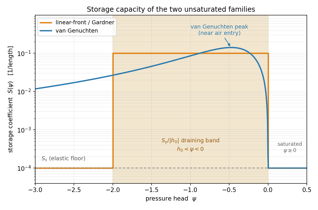
The storage coefficient \(S(\psi)\): a constant elastic floor \(S_s\) plus a drainage capacity — a boxcar band for the linear-front / Gardner model, and a smooth peak near air entry for van Genuchten.

Time stepping

The theta method

The semi-discrete system is advanced in time with the theta method. Over a step from \(t\) to \(t + \Delta t\), writing \([M]/\Delta t\) for the storage matrix scaled by the step size,

\(\left(\dfrac{[M]}{\Delta t} + \theta[K]\right)\{h\}_{t+\Delta t} = \dfrac{[M]}{\Delta t}\{h\}_{t} + \{Q\} - (1-\theta)[K]\{h\}_{t}\)

The weight \(\theta\) selects the scheme: \(\theta = 1\) is backward Euler, the default — unconditionally stable and free of the oscillations that dog explicit and centered schemes on sharp infiltration fronts. \(\theta = 0.5\) is Crank–Nicolson, second-order accurate in time but more prone to ringing on rapidly switching boundaries. Backward Euler is recommended for slope-stability work.

Picard iteration

Because both \([K]\) (through \(k_r\)) and \([M]\) (through \(S\)) depend on the head field being solved for, each step is nonlinear and is resolved by Picard iteration. Within a step the conductivity matrix is rebuilt from the current head iterate's \(k_r\) and the mass matrix is rescaled by the current \(S\), the linear system above is solved, and the process repeats until the maximum nodal head change between successive iterates falls below a tolerance (scaled by a characteristic head span). For an unconfined problem the exit-face active set (below) must also settle before the step is accepted.

Adaptive time stepping

The step size \(\Delta t\) is chosen adaptively so that the solver takes small steps through rapid transients and large steps through quiescent periods:

• Head-change limiter. A step is rejected and halved whenever the largest head change at any free node exceeds a fraction (default 5%) of the characteristic head span. This resolves sharp fronts. The change at Dirichlet nodes is deliberately excluded — a stepped reservoir level jumps by its full amount regardless of \(\Delta t\), and counting it would drive the step size to its floor for no benefit.
• Convergence-based growth. After a step that converges easily (few Picard iterations) the next step grows by a fixed factor; after a step that needed many iterations it shrinks. A step that fails to converge is halved and retried down to a minimum step size, at which point the last iterate is force-accepted (and the run flagged non-converged) so the march always makes progress.
• Schedule clamping. The step size is always clamped so the stepper lands exactly on every saved time (see Outputs). Saved frames are therefore computed states, never interpolated between steps.

Lumped mass

The storage matrix is lumped (diagonalized) rather than kept in its full consistent form. A consistent mass matrix couples neighboring nodes and can produce non-physical overshoot and undershoot — spurious pressure oscillations — ahead of a steep wetting front; lumping suppresses this and keeps each step's system well-behaved. XSLOPE uses HRZ (special lumping) diagonal scaling, which coincides with simple row-summing on linear elements and stays strictly positive on quadratic elements. Lumped mass is the default and only option in the current release.

Boundary conditions

A transient run reuses the steady boundary-condition types — specified head, exit face, and specified flux — and adds the ability to drive any of them from a time series rather than a constant.

Time series

A specified-head or specified-flux value on the seep bc sheet may be a number (as in a steady model) or the name of a series defined on the tseep sheet. The tseep sheet holds a single shared time column and up to five named series (the template ships default headers t1…t5, renamable to anything short). One series can drive several boundaries, and each referencing block's own type — head, reservoir, or flux — decides whether the series numbers are read as a plain Dirichlet head, a submerged-only reservoir level, or a specified flux.

Each series is a curve of value versus time with these breakpoint semantics:

• Values are interpolated linearly between the times at which the series has entries.
• The series is held constant before its first entry and after its last.
• A blank cell between entries means "no breakpoint here" — the series interpolates straight through it — so independent series with different breakpoints share the one time column.
• A step change is entered by repeating a time on two consecutive rows with different values; the new value applies from that time onward (the series is right-continuous at the step).

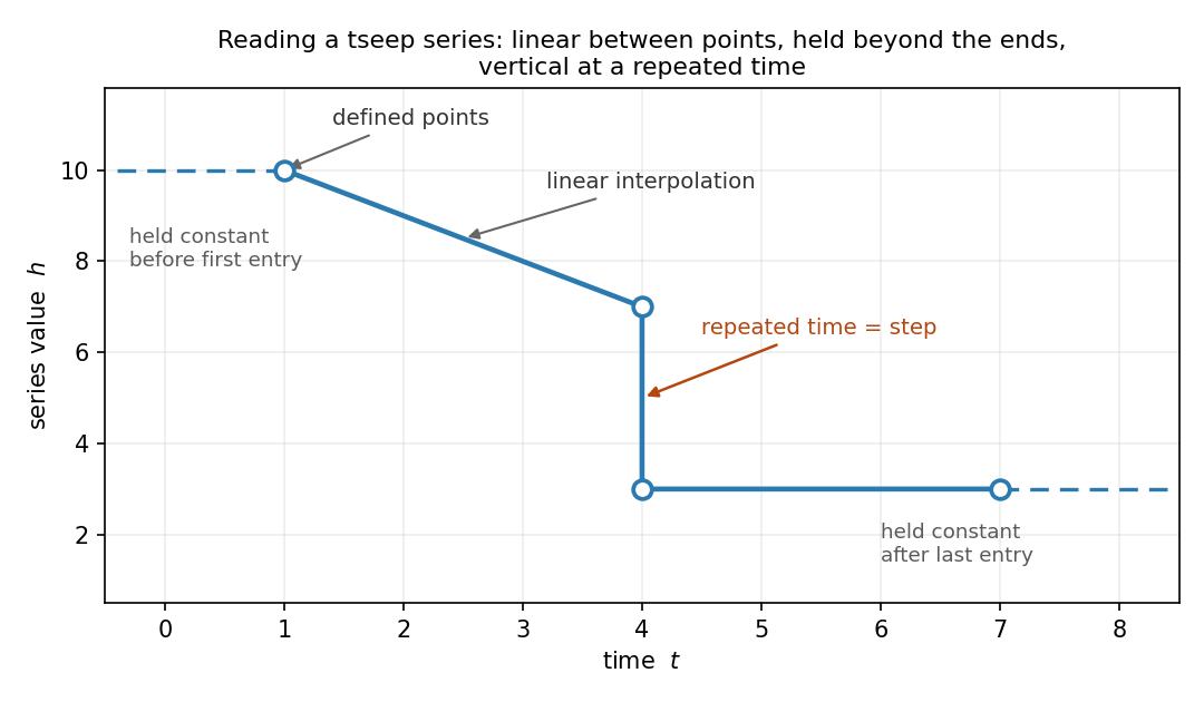
A tseep series runs linearly between its defined points, holds constant beyond the first and last, and steps vertically wherever a time is repeated.

Numeric fluxes are baked into the load vector once; a series-driven flux is assembled once as a unit-flux load vector for its polyline and scaled by the series value each step, since the flux load is linear in its value.

Head types: head and reservoir

A Dirichlet boundary comes in two named types, chosen per block in the seep bc sheet's type cell. They differ only in how a value above the applied level is treated; for a value drawn at or below the level (the usual case) they are identical.

A head boundary is a plain Dirichlet: every node of the polyline is held at the value — constant or series \(h(t)\) — at all times. It can hold a negative-pressure (suction) head and it never converts to an exit face. This is the type for a drained face, a specified-suction laboratory boundary, or any imposed head that should be enforced regardless of elevation.

A reservoir boundary is the submerged-only Dirichlet used for a reservoir or tailwater whose level rises and falls. At each time \(t\), a node on the boundary is held at the level \(h(t)\) only while it is submerged — its elevation is at or below \(h(t)\). A node that the falling water level has left above the waterline is not held at a head; instead it is converted to an exit-face node, free to seep. The physical motivation is that a face the water level has just exposed does not become a no-flow boundary: the soil behind it is still saturated, and that water can seep back out through the newly unsubmerged surface. Pinning such nodes to the (now lower) reservoir level or sealing them would both misstate the physics. As the level moves, nodes cross between the two regimes and the exit point migrates up and down the face — which is precisely the behavior a drawdown demands. (A constant numeric reservoir level behaves the same way: nodes above the level become exit faces, so draw the face only up to the level unless that migration is intended.)

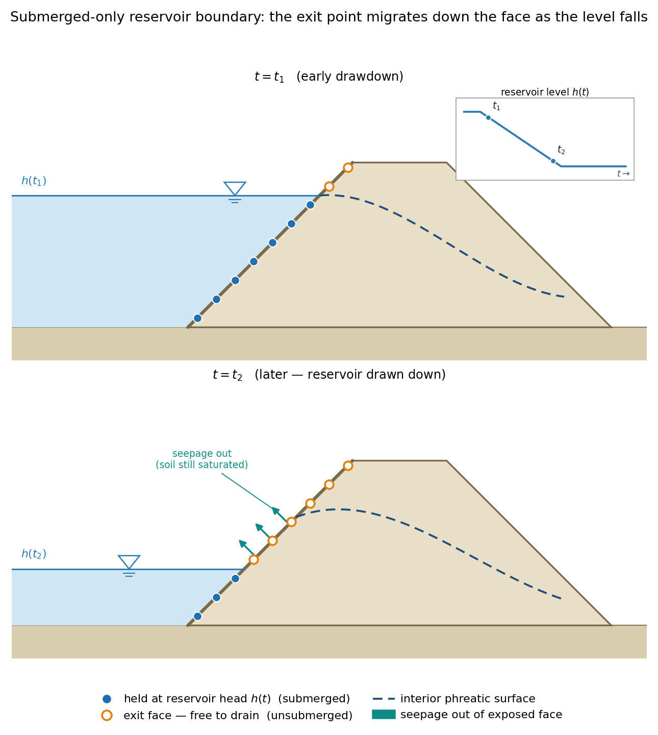
As the reservoir level falls from \(h(t_1)\) to \(h(t_2)\), face nodes the water leaves above the line switch from held reservoir head to exit face, and the still-saturated soil drains back out through the newly exposed surface.

Exit-face behavior

The exit face itself — whether present statically as a downstream seepage face or appearing dynamically as a reservoir head falls below a node — is resolved each step with the same SEEP2D-style active-set rule the steady solver uses: a boundary node is held saturated (at atmospheric pressure) unless the head would fall below its elevation or the boundary reaction would have to push water into the domain, in which case it is released to no-flow. On quadratic meshes (tri6, quad8, quad9) each seepage-face edge is tracked all-or-nothing across its corner and midside nodes — the same edge treatment the steady solver applies — so the transition point lands cleanly on a corner and the element order of a transient run is unrestricted.

Initial conditions

Marching in time requires a head field at \(t = 0\) to start from. By default XSLOPE computes it as a steady solve at the \(t = 0\) boundary configuration: the boundary series are evaluated at \(t = 0\), and the ordinary steady solver is run — a single linear solve for a confined problem, or the steady exit-face Picard solver for an unconfined one. This gives a physically consistent starting field that is already in equilibrium with the initial boundaries, so the transient march begins from a genuine steady state rather than an arbitrary guess. An explicit initial head field may be supplied instead when one is known.

The repeated-time idiom for a steady starting state. Because the initial condition is a steady solve at the \(t = 0\) boundaries, the way to start a run from a particular steady state — a full reservoir before drawdown, say — is simply to give the driving series that value at \(t = 0\). The \(t = 0\) steady solve then reproduces the full-reservoir flow field. To hold that state briefly and then change it, use a step (a repeated time): the series sits at the initial value through \(t = 0\), so the steady initial condition is unaffected, and then steps or ramps to the new value at a later time. This is the standard setup for rapid drawdown — a steady full-pool initial condition followed by a scheduled lowering.

Outputs

Saved-frame schedule

The solver does not store every computed step — it stores a curated set of saved frames. The saved times are the union of

• the save_interval grid (a uniform spacing; defaults to roughly 50 frames over the duration when left blank),
• any explicit save_times listed on the tseep sheet,
• the rapid-drawdown stage_1 / stage_2 times, and
• every series breakpoint,

all clamped to the interval \((0, \text{duration}]\), de-duplicated and sorted. The \(t = 0\) initial condition is always saved as the first frame. Because the adaptive stepper is clamped to land exactly on each of these times, every saved frame is a computed state.

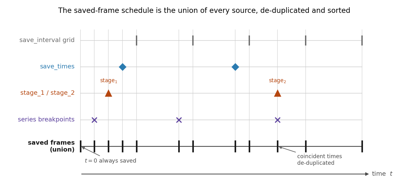
The saved-frame schedule is the union of the save_interval grid, explicit save_times, the stage times, and every series breakpoint — de-duplicated, sorted, and always including \(t = 0\).

Files

export_transient_solution writes two files:

• {base}_tseep.csv — a long-format table with one block of n_nodes rows per saved frame, columns time, node_id, head, u. Velocities are deliberately not stored; they are derived on load (below). No stream function is stored either: a transient frame has no flow net (see the note below), so a per-frame flow-function solve would be meaningless to draw — dropping it keeps the file lean and speeds up the export. (A legacy 5-column file that still carries a phi column loads fine; the extra column is ignored.)
• {base}_tseep_meta.json — the frame ledger: saved times, node count, unit system and time unit, the theta/lumped provenance, the dt history, the per-frame inflow/outflow, the mass-balance ledger, the stage times, and the source input/mesh file names.

Per-frame outputs, and why inflow ≠ outflow

Each saved frame reports separate inflow and outflow totals, computed at solve time. Under storage exchange these differ — the difference is exactly the water being stored in, or released from, the soil at that instant. A steady solution's single "Total Flowrate" no longer applies; a transient frame reports both rates, and the frame title carries them beneath the frame time.

Derive-on-load velocities

When a saved frame is read back (import_transient_solution), the velocity and hydraulic gradient fields are recomputed from the stored head, the mesh, and the (possibly \(k_r\)-scaled) conductivity — the same derivation the steady solver uses. Storing only head and pressure keeps the file compact, and reconstructing the derived fields on load reproduces exactly what a steady solve would report for that head field. Each reconstructed frame is a full solution dict that plot_seep_solution renders unchanged.

Mass-balance ledger

The meta file records a running mass-balance ledger. The cumulative net boundary inflow (the discrete storage change the solve actually applied) is compared, at each saved frame, against an independent secant estimate of the change in stored water — the integral of a storage-potential function \(\Phi(\psi)\) over the domain, in the mass-conservative mixed-form spirit of Celia et al. (1990). Their difference, normalized to the storage scale, is the reported closure. For a saturated linear problem the two agree to machine precision; a growing closure error on a strongly nonlinear run is the signal to tighten the step controls.

Rapid drawdown staging

A transient run couples directly to a rapid-drawdown stability analysis. The tseep controls carry two optional stage times, stage_1 and stage_2 (with stage_1 < stage_2) — for example, the full-reservoir steady state at stage_1 and the drawn-down state at stage_2. Both times are forced into the saved-frame schedule, so each is a computed frame.

stage_transient_for_drawdown then pulls those two frames in memory — no intermediate files — and places their pore-pressure fields into slope_data['seep_u'] and slope_data['seep_u2'], which are exactly the structures the classic two-steady-file drawdown path produces. The existing three-stage rapid-drawdown machinery then runs unchanged. When a transient solution with stage times is present it takes precedence over the classic {base}_seep.csv / {base}_seep2.csv files; a model without stage times continues to use the classic path.

See the Rapid Drawdown Analysis page for the stability methodology the staged pore pressures feed.

Studio

Transient seepage can be prepared and run without writing code in XSlope Studio: edit the time series, save schedule, and stage times in the Transient inputs editor (Inputs → Transient), set the storage properties, build a mesh, and run the analysis from the seepage tools — the run reports determinate progress and can be cancelled — then step through the saved frames in the solution view. See Studio → Running Analyses → Seepage.

Code Examples and Usage

Running a transient analysis

from xslope.fileio import load_slope_data
from xslope.mesh import build_polygons, build_mesh_from_polygons
from xslope.seep import (
    build_seep_data, build_tseep_data, run_transient_seepage,
    export_transient_solution,
)

# Load a model whose workbook carries a filled-in tseep sheet and Ss/Sy storage
slope_data = load_slope_data("inputs/slope/dam_drawdown.xlsx")

# Mesh (any element order; quadratic tri6 resolves exit faces per step too)
polygons = build_polygons(slope_data)
mesh = build_mesh_from_polygons(polygons, target_size=2.0, element_type='tri3')

# Steady-style seep data (carries storage + BC series bindings) + transient controls
seep_data = build_seep_data(mesh, slope_data)
tseep_data = build_tseep_data(slope_data)   # None if the file has no tseep sheet

# March in time (backward Euler by default)
solution = run_transient_seepage(seep_data, tseep_data)
print(f"Saved {len(solution['frames'])} frames over duration {solution['duration']}")
print(f"Mass-balance closure at end: {solution['mass_balance']['final_closure']:.2e}")

# Write the run to {base}_tseep.csv (+ _tseep_meta.json)
export_transient_solution(
    seep_data, solution, "outputs/dam_drawdown",
    input_file="inputs/slope/dam_drawdown.xlsx",
)

Reloading a saved run and plotting a frame

from xslope.seep import import_transient_solution, transient_frame_index
from xslope.plot_seep import plot_seep_solution

# Reconstruct the solution (velocities/gradients derived on load)
ts = import_transient_solution(seep_data, "outputs/dam_drawdown")

# Pick the frame nearest a time (must be a saved time)
i = transient_frame_index(ts, 10.0)
frame = ts["frames"][i]          # a full solution dict plot_seep_solution consumes
print(f"Frame t={frame['time']}: inflow={frame['inflow']:.4g}, "
      f"outflow={frame['outflow']:.4g}")

plot_seep_solution(
    seep_data, frame,
    levels=20, phreatic=True, fill_contours=True, mesh=True,
)

Coupling to rapid drawdown

from xslope.seep import run_transient_seepage, stage_transient_for_drawdown

# tseep controls must set stage_1 and stage_2 (stage_1 < stage_2)
solution = run_transient_seepage(seep_data, tseep_data)

# Pull the two stage frames in memory into slope_data['seep_u'] / ['seep_u2']
slope_data = stage_transient_for_drawdown(slope_data, solution)

# slope_data is now ready for the three-stage rapid_drawdown analysis

For a single-time stability analysis at one frame, select_transient_frame_u(slope_data, solution, time=...) places that frame's pore pressures into slope_data['seep_u'] for the ordinary u = seep machinery.

Verification and Examples

The transient solver is exercised from two directions. A verification tier checks the marched head and pressure fields — and, where a drawdown history drives stability, the factor of safety through time — against published closed-form, vendor, and imported-field solutions. A set of worked examples then carries a complete transient input file from geometry through a saved-frame solution, and on into a rapid-drawdown stability check. Each links back here for the formulation, and this page links out to both.

Verification

The transient rows in the corpus own their own numbers; each page below is entered at its transient section:

• Rocscience Slide2 groundwater — transient problems: the Terzaghi / Ferris / Pyrah consolidation columns and the earth-dam and lagoon seepage runs (GW15–GW21, all built), locked against closed-form or recomputed-analytical targets.
• GeoStudio SEEP/W transient seepage: the consolidation, infiltration, reservoir-drawdown, clay-lined-pond, leach-column, and stepped-suction examples (SEEPW-T01–T05 and T07 built), with the multi-layer infiltration case (T06) documented as blocked and why.
• RS2 earth dam under transient unsaturated seepage: the RS2-67 SSRM family, driven both by RS2's own imported 90 h drawdown pore-pressure field and by XSLOPE's own transient-flow reconstruction locked as an own-flow regression.
• Rocscience Slide2 — VP102: a rapid-drawdown earth dam whose factor of safety is tracked across the 60–1500 h drawdown from a single uncoupled transient seepage solve.

Worked examples

These sample problems build a transient run end to end from an input file you can download and open:

• Earth Dam — Reservoir Drawdown: a homogeneous dam followed through a reservoir drawdown driven by a falling reservoir series.
• Johnson Reservoir — Zoned Drawdown: the zoned Johnson Reservoir dam drawn down over 45 days, with stage_1 / stage_2 set for rapid drawdown.
• Rapid drawdown from a transient solution: the Johnson Reservoir drawdown carried into a three-stage rapid-drawdown stability analysis, reading its two stage frames from the one transient history.

References

Celia, M.A., Bouloutas, E.T., & Zarba, R.L. (1990). A general mass-conservative numerical solution for the unsaturated flow equation. Water Resources Research, 26(7), 1483-1496. https://doi.org/10.1029/WR026i007p01483

Freeze, R.A., & Cherry, J.A. (1979). Groundwater. Prentice-Hall.

Gardner, W.R. (1958). Some steady-state solutions of the unsaturated moisture flow equation with application to evaporation from a water table. Soil Science, 85(4), 228-232.

van Genuchten, M.Th. (1980). A closed-form equation for predicting the hydraulic conductivity of unsaturated soils. Soil Science Society of America Journal, 44(5), 892-898. https://doi.org/10.2136/sssaj1980.03615995004400050002x