Seepage - Slope Stability Integration
Effective Stress and the Role of Pore Pressure
Slope stability analysis for saturated or partially saturated soils requires an understanding of the relationship between total stress, effective stress, and pore water pressure. The shear strength of soil — and therefore the stability of a slope — is governed by effective stress, not total stress.
Terzaghi's effective stress principle states that the effective stress \(\sigma'\) is the difference between the total stress \(\sigma\) and the pore water pressure \(u\):
\(\sigma' = \sigma - u\)
The shear strength of soil is described by the Mohr-Coulomb failure criterion, expressed in terms of effective stress:
\(\tau_f = c' + \sigma'_n \tan \phi'\)
where:
- \(\tau_f\) is the shear strength at failure
- \(c'\) is the effective cohesion
- \(\phi'\) is the effective friction angle
- \(\sigma'_n\) is the effective normal stress on the failure plane
Substituting Terzaghi's effective stress relationship:
\(\tau_f = c' + (\sigma_n - u) \tan \phi'\)
This equation makes clear that pore water pressure \(u\) directly reduces the effective normal stress acting on a potential failure surface, which in turn reduces the available shear strength. As pore pressures increase — for example due to rainfall infiltration, rising reservoir levels, or seepage through an embankment — the effective stress decreases and the factor of safety against slope failure is reduced. Accurate determination of the pore pressure distribution within a slope is therefore essential for a reliable stability assessment.
For simple groundwater conditions, pore pressures can be estimated from a piezometric line. However, for slopes with complex seepage patterns — such as earth dams, levees, or slopes adjacent to reservoirs — a finite element seepage analysis provides a much more accurate representation of the pore pressure field throughout the domain.
Computing Pore Pressure from Seepage Analysis
The primary output of seepage analysis is the hydraulic head distribution throughout the analysis domain. However, slope stability analysis requires pore pressure values rather than hydraulic heads. The conversion between these quantities follows the fundamental relationship:
\(u = \gamma_w (h - z)\)
where: - \(u\) is the pore water pressure - \(\gamma_w\) is the unit weight of water (typically 9.81 kN/m³ or 62.4 lbf/ft³) - \(h\) is the hydraulic head from seepage analysis - \(z\) is the elevation coordinate
This relationship automatically accounts for the effect of elevation on pore pressure while preserving the hydraulic gradients computed by the seepage analysis. Positive pore pressures indicate groundwater under pressure (below the phreatic surface), while zero or negative values indicate conditions above the groundwater table.
Overview
The seepage analysis tools in XSLOPE can be used independently to simulate flow through porous media for a broad variety of applications. However, the seepage analysis tools can also be used in conjunction with the slope stability analysis tools. Since both seepage and slope stability analysis use the same input file and the same approach to defining material properties and model geometry, integrating the two analysis tools is straightforward. The same Excel input template is used for both analyses. The seepage analysis is performed first and the seepage solution, including pore pressures at nodes, is saved to a set of files. The mesh and seepage solution files are then automatically imported when the Excel input file is loaded. The seepage results can be used to define pore pressures for both limit equilibrium method (LEM) and finite element method (FEM) slope stability analyses. Each step of this process is described in detail below.
Saving the Seepage Solution
After performing the seepage analysis, the seepage solution should be saved to a set of two files. The first is a JSON file containing the 2D finite element mesh including both nodal coordinates and element topology. The second file is a CSV file containing the seepage solution, including hydraulic heads, pressure head, pore pressures, and total head at each node. The seepage solution files should be saved using a specific naming convention. If the input file is named myfile.xlsx, the seepage files should be exported as myfile_mesh.json and myfile_seep.csv. In other words, the prefix of the input file should be used as the prefix for the seepage files and they should end with the suffix _mesh.json and _seep.csv. The seepage solution files are saved in the same folder as the Excel input template.
The following code snippet shows a complete workflow for building a mesh, running a seepage analysis, and saving both the mesh and solution files:
from pathlib import Path
from xslope.fileio import load_slope_data
from xslope.mesh import build_polygons, build_mesh_from_polygons, export_mesh_to_json
from xslope.plot_seep import plot_seep_data, plot_seep_solution
from xslope.seep import build_seep_data, run_seepage_analysis, export_seep_solution

input_file = "docs/seep/files/xslope_johnson_res.xlsx"
input_path = Path(input_file)

slope_data = load_slope_data(input_file)

element_type = 'tri6'
re_mesh = True

# Use existing mesh from slope_data if available, otherwise build a new one
if slope_data.get("mesh") is not None and not re_mesh:
    print("Using existing mesh file.")
    mesh = slope_data["mesh"]
else:
    print("Building new mesh from profile line data.")
    polygons = build_polygons(slope_data)
    x_range = [min(x for x, _ in slope_data['ground_surface'].coords),
               max(x for x, _ in slope_data['ground_surface'].coords)]
    target_size = (x_range[1] - x_range[0]) / 60
    mesh = build_mesh_from_polygons(polygons, target_size, element_type)
    mesh_file = input_path.parent / f"{input_path.stem}_mesh.json"
    export_mesh_to_json(mesh, mesh_file)

# Build seep data and run seepage analysis
seep_data = build_seep_data(mesh, slope_data)
plot_seep_data(seep_data, show_nodes=True, show_bc=True)

solution = run_seepage_analysis(seep_data, tol=1e-4)
plot_seep_solution(seep_data, solution, variable="head", flowlines=True, phreatic=True)

# Save the seepage solution to CSV
seep_file = input_path.parent / f"{input_path.stem}_seep.csv"
export_seep_solution(seep_data, solution, seep_file)
Note that the Path class from Python's pathlib module is used to construct the output file paths. The input_path.stem property extracts the filename without the extension, and the input_path.parent property provides the directory. This ensures the mesh and solution files are saved in the same directory as the input file with the correct naming convention.
When a mesh file already exists (e.g., it was previously exported or included alongside the Excel template), load_slope_data() will automatically import it and store it under slope_data["mesh"]. The re_mesh flag controls whether to rebuild the mesh from scratch or reuse the existing one. Setting re_mesh = False skips mesh generation and uses the pre-built mesh, which is useful when iterating on boundary conditions or seepage parameters without needing to regenerate the mesh.
Rapid Drawdown Analysis
The input template is set up to allow the specification of two sets of boundary conditions for the seepage analysis.
These are stored in the seep bc sheet and the seep bc (2) sheet. The first set is used for a typical seepage
analysis, but when conducting a rapid drawdown analysis, the first set of boundary conditions can be used to simulate
the full reservoir condition and the second set of boundary conditions can be used to simulate the drawn-down
condition. Both of the solutions can then be imported to define pore pressures for both the full reservoir and
drawn-down conditions when performing slope stability analysis. When performing the seepage analysis, both solutions
should be found using the same mesh geometry. Then a single mesh file is exported in JSON format and the two
solutions are exported in CSV format. The second seepage solution should be saved with a _seep2.csv extension. The
following code snippet shows how to export the seepage solution files for the case with rapid drawdown:
from pathlib import Path
from xslope.fileio import load_slope_data
from xslope.mesh import build_polygons, build_mesh_from_polygons, export_mesh_to_json
from xslope.plot_seep import plot_seep_data, plot_seep_solution
from xslope.seep import build_seep_data, run_seepage_analysis, export_seep_solution

input_file = "docs/inputs/slope/xslope_lface.xlsx"
input_path = Path(input_file)
slope_data = load_slope_data(input_file)

element_type = 'tri6'
re_mesh = True

# Use existing mesh or build a new one
if slope_data.get("mesh") is not None and not re_mesh:
    mesh = slope_data["mesh"]
else:
    polygons = build_polygons(slope_data)
    x_range = [min(x for x, _ in slope_data['ground_surface'].coords),
               max(x for x, _ in slope_data['ground_surface'].coords)]
    target_size = (x_range[1] - x_range[0]) / 60
    mesh = build_mesh_from_polygons(polygons, target_size, element_type)
    mesh_file = input_path.parent / f"{input_path.stem}_mesh.json"
    export_mesh_to_json(mesh, mesh_file)

# First boundary condition (e.g., full reservoir)
seep_data = build_seep_data(mesh, slope_data)
solution = run_seepage_analysis(seep_data, tol=1e-4)
plot_seep_solution(seep_data, solution, variable="head", flowlines=True, phreatic=True)

seep_file = input_path.parent / f"{input_path.stem}_seep.csv"
export_seep_solution(seep_data, solution, seep_file)

# Second boundary condition (e.g., drawn-down reservoir)
if slope_data.get("has_seepage_bc2"):
    seep_data2 = build_seep_data(mesh, slope_data, seep_bc=2)
    solution2 = run_seepage_analysis(seep_data2, tol=1e-4)
    plot_seep_solution(seep_data2, solution2, variable="head", flowlines=True, phreatic=True)

    seep_file2 = input_path.parent / f"{input_path.stem}_seep2.csv"
    export_seep_solution(seep_data2, solution2, seep_file2)
The has_seepage_bc2 key in slope_data is set automatically by load_slope_data() when the input Excel file contains a seep bc (2) sheet with valid boundary condition data. The seep_bc=2 argument to build_seep_data() tells it to use the second set of boundary conditions instead of the default first set. Note that both analyses use the same mesh — only the boundary conditions change.
Automatic Import of Seepage Files
When XSLOPE reads an Excel input file via load_slope_data(), it automatically checks to see if a set of seepage files exists for the simulation. It does this by looking for files in the same directory and with the same prefix as the Excel input file, ending with the suffixes _mesh.json, _seep.csv, and _seep2.csv. If the mesh file exists, it is imported and stored in the slope_data dictionary under the "mesh" key. If any materials have their pore pressure option set to seep, the seepage solution CSV files are also imported and the nodal pore pressures are stored under the "seep_u" and "seep_u2" keys. No additional code is required to import these files — simply calling load_slope_data() handles the import automatically, provided the files follow the naming convention.
For example, given the following set of files in the same directory:
xslope_johnson_res_lem.xlsx
xslope_johnson_res_lem_mesh.json
xslope_johnson_res_lem_seep.csv
Calling load_slope_data("xslope_johnson_res_lem.xlsx") will automatically import the mesh and seepage solution alongside the Excel data.
Using Zip Archives (Colab Notebook)
The Colab seepage notebook supports uploading a zip archive instead of a standalone Excel file. This is convenient when you want to bundle an Excel input template with a pre-built mesh file (and optionally existing seepage solution files) so that everything can be uploaded in a single step.
Uploading a Zip Archive
When a .zip file is uploaded, the notebook extracts its contents and automatically locates the .xlsx file inside:
from google.colab import files
import zipfile

upload = files.upload()
file_name = list(upload.keys())[0]

if file_name.endswith('.zip'):
    with zipfile.ZipFile(file_name, 'r') as zip_ref:
        zip_ref.extractall()
        for f in zip_ref.namelist():
            if f.endswith('.xlsx'):
                file_name = f
                break
After extraction, the mesh JSON file (if included) will be in the working directory alongside the Excel file. When load_slope_data() is called, it will automatically detect and import the mesh file using the standard naming convention.
Downloading Results as a Zip Archive
After running the seepage analysis, the notebook packages all output files — the original Excel file, the mesh JSON, and the seepage solution CSV(s) — into a results zip archive for download:
import zipfile
from pathlib import Path

input_path = Path(file_name)
zip_file_name = f"{input_path.stem}_results.zip"

with zipfile.ZipFile(zip_file_name, 'w') as zipf:
    zipf.write(file_name)                                # Original Excel file
    zipf.write(f"{input_path.stem}_mesh.json")           # Mesh file
    zipf.write(f"{input_path.stem}_seep.csv")            # Seepage solution
    if slope_data.get("has_seepage_bc2"):
        zipf.write(f"{input_path.stem}_seep2.csv")       # Second BC solution

files.download(zip_file_name)
This results zip can then be re-uploaded in a future session to continue analysis with the pre-built mesh, avoiding the need to regenerate it.
Selecting the SEEP Option for Pore Pressure Calculation
When performing a slope stability analysis, a set of shear strength parameters and a pore pressure option are entered for each material. The pore pressure options are as follows:
| Option | Description |
|---|---|
| none | No pore pressures. This is appropriate for dry soils or total stress analysis |
| piezo | Pore pressures are derived from a piezometric line defined on the piezo tab |
| seep | Pore pressures are derived from the results of a 2D finite element seepage analysis |
For the seep option, the user first performs a seepage analysis as described above and exports the resulting finite
element mesh and solution file using the specified naming convention. For a rapid drawdown analysis, one mesh file
and two solution files are exported.
Conservative Treatment of Negative Pore Pressures
In certain situations, the seepage analysis may compute negative pore pressures (tensions) in portions of the domain, particularly in unsaturated zones or regions with strong capillary effects. While these negative pore pressures may be physically realistic, their inclusion in slope stability analysis can lead to unconservative results by artificially increasing effective stresses and apparent slope stability.
XSLOPE implements a conservative approach by automatically setting any computed negative pore pressures to zero before transferring them to slope stability calculations. This treatment ensures that:
Conservative Assessment: Slope stability calculations do not benefit from potentially unreliable tensile strength in pore water Physical Realism: Avoids dependence on soil-water tension effects that may not persist under loading conditions Robustness: Eliminates sensitivity to uncertain unsaturated soil parameters that may not be well-characterized
Using Seepage Results with LEM Analysis
For limit equilibrium slope stability analysis, the mesh and seepage solution define the pore pressure field used to compute effective stresses. When the pore pressure option is set to seep for a given material, pore pressures from the seepage solution are interpolated to the base of each slice that passes through that material. Materials with other pore pressure options (e.g., none or piezo) are unaffected by the seepage data and continue to use their specified pore pressure method.
Interpolation to Slice Locations
The integration of seepage analysis results with limit equilibrium slope stability calculations requires interpolation of pore pressures from the seepage mesh nodes to the base center of each slice used in limit equilibrium analysis. XSLOPE implements a robust interpolation scheme that preserves the accuracy of the computed pore pressure field while ensuring computational efficiency.
The interpolation process follows these key steps:
Spatial Search: For each slice base center, the system identifies the seepage analysis element containing that point using efficient spatial search algorithms.
Shape Function Evaluation: The pore pressure at the slice base center is computed using the finite element shape functions and the nodal pore pressure values of the containing element:
\(u(x,y) = \sum_{i=1}^{n} N_i(x,y) \cdot u_i\)
where \(N_i\) are the element shape functions and \(u_i\) are the nodal pore pressures.
Using Seepage Results with FEM Analysis
For finite element slope stability analysis using the Shear Strength Reduction Method (SSRM), the seepage solution provides two things:
-
Mesh geometry: The finite element mesh from the seepage analysis is used directly as the mesh for the FEM slope stability analysis. The mesh should not be rebuilt for the FEM analysis. Both the seepage and FEM solutions must be based on the same mesh to ensure consistency of the pore pressure field with the stress analysis domain.
-
Pore pressures: For all materials where the pore pressure option is set to
seep, the nodal pore pressures from the seepage solution are applied as effective stress pore pressures in the FEM analysis. As with LEM, materials using other pore pressure options are unaffected.
Interpolation of Pore Pressures to Gauss Points
In the FEM formulation, stresses are evaluated at Gauss (integration) points within each element. To incorporate pore pressure effects into the effective stress calculation, the nodal pore pressures from the seepage solution must be interpolated to each Gauss point. This is done using the same element shape functions \(N_i\) that are used for displacement interpolation:
\(u_{gp} = \sum_{i=1}^{n} N_i \cdot u_i\)
where \(u_i\) are the nodal pore pressures and \(N_i\) are the shape function values evaluated at the Gauss point's natural coordinates. These interpolated pore pressures are precomputed once during the setup phase (build_fem_data) and stored for each Gauss point, so they do not need to be recalculated during the viscoplastic iteration loop.
At each Gauss point, the Mohr-Coulomb yield function is evaluated using the effective mean stress:
\(\bar{\sigma}' = \bar{\sigma} - u_{gp}\)
\(F = \tau_{max} - \bar{\sigma}' \sin\phi - c \cos\phi\)
where \(\bar{\sigma} = (\sigma_x + \sigma_y)/2\) is the total mean normal stress and \(\tau_{max}\) is the maximum shear stress at the Gauss point. A positive value of \(F\) indicates that the stress state has exceeded the Mohr-Coulomb yield surface and plastic correction is required. By reducing the effective stress, positive pore pressures shrink the elastic domain and make yielding more likely — consistent with the physical effect of pore pressure on soil strength.
Negative pore pressures (suction) are clamped to zero before interpolation, consistent with the conservative treatment described earlier.
Element Type Considerations for FEM
When building a seepage mesh that will later be used for FEM slope stability analysis, it is important to use quadratic elements (tri6, quad8, or quad9) for the seepage mesh. Linear elements (tri3 and quad4) suffer from volumetric locking in the elastic-plastic FEM analysis, causing them to significantly overestimate the factor of safety. Since both analyses must share the same mesh, the element type must be chosen with the FEM requirements in mind.
See Element Type Selection and Volumetric Locking for a detailed discussion of element types, locking behavior, and benchmark results.
Example Problem
The follow example illustrates this process. The following problem corresponds to the Johnson Reservoir problem from the Sample Problems - Seepage Analysis page. The input file for this problem can be found here:
This input file contains all of the inputs for a seepage analysis, a limit equilibrium (LEM) slope stability analysis, and a finite element (FEM) slope stability analysis. The input plot for the seepage analysis is as follows:
The inputs are used to build a mesh with quadratic triangular (tri6) elements. The seepage solution is as follows:
After running the seepage analysis, two additional files were created:
xslope_johnson_res_mesh.json <--- mesh file
xslope_johnson_res_seep.csv <--- seepage solution file with pore pressures
The Excel file is then loaded for a LEM analysis, and the inputs are plotted again:
Note the mesh display in the background. This indicates that the mesh file and the seep solution file are automatically loaded when the Excel file is imported. These two files are used to define pore pressures for the LEM analysis. In this case, all three materials have the 'seep' option selected for pore pressures in the materials table. A critical-circle search with Spencer's method gives FS = 1.25:
Finally, the same Excel file and the corresponding mesh and seepage solution files are imported again for a FEM slope stability analysis. The pore pressures from the seepage solution are interpolated to every Gauss point and enter the analysis through the effective-stress formulation (see FEM Overview), so the FEM uses exactly the same pore pressure field as the LEM analysis, and the reservoir water above the submerged upstream face is applied as a consistent boundary pressure. The shear strength reduction method (SSRM) is run with the default non-convergence criterion. The result is FS = 1.25, and the plots below show the solution at the computed factor of safety:
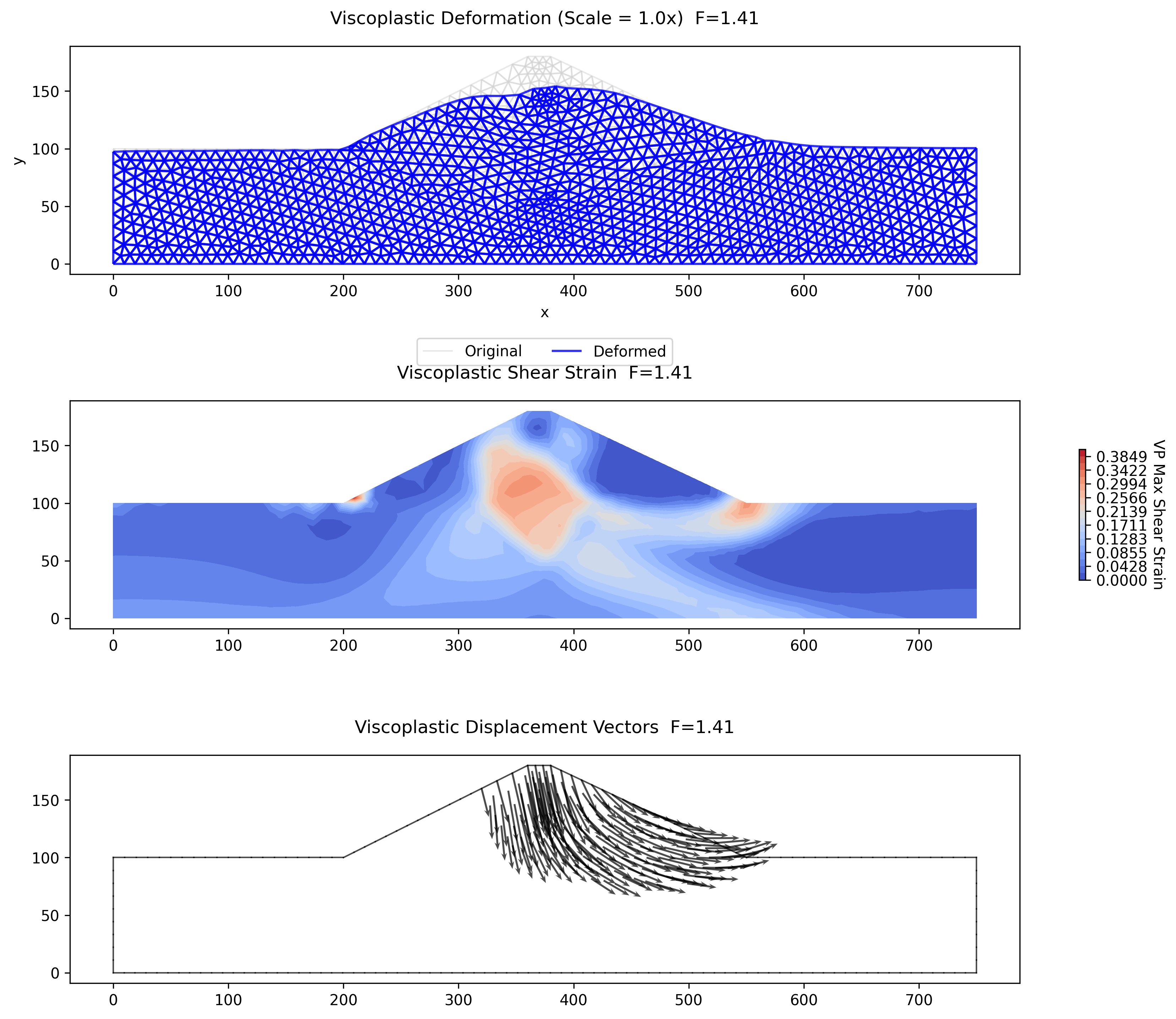
The deformed mesh and displacement vectors show a deep-seated mechanism through the embankment and into the foundation, consistent with the critical circle found by the LEM search. The FEM factor of safety of 1.25 agrees with the Spencer's method result of 1.25 to within about 1% — typical of the agreement between SSRM and a well-converged limit equilibrium solution when both use the same strength and pore pressure inputs. Since neither method depends on the other (the LEM prescribes a circular surface, while the FEM develops the failure mechanism from the stress field alone), this agreement provides a strong mutual check on the combined seepage and slope stability workflow.
Piezometric Line vs. Seepage-Derived Pore Pressures
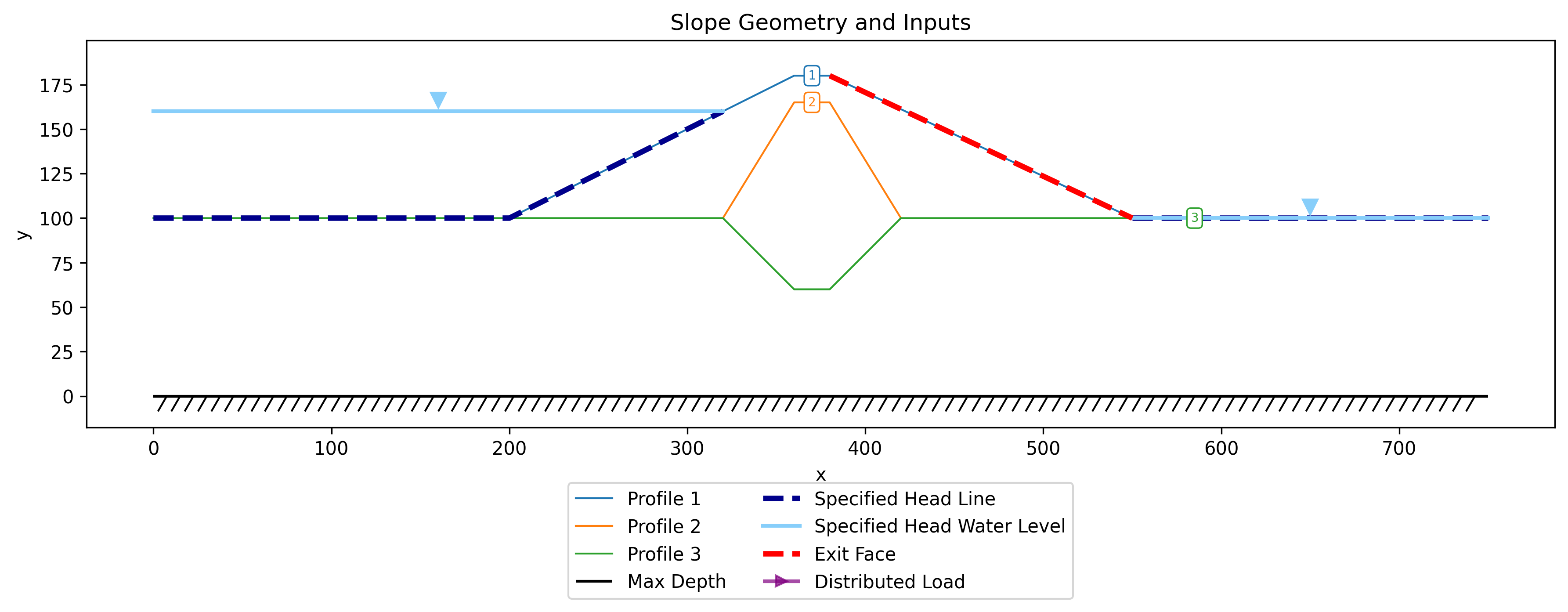
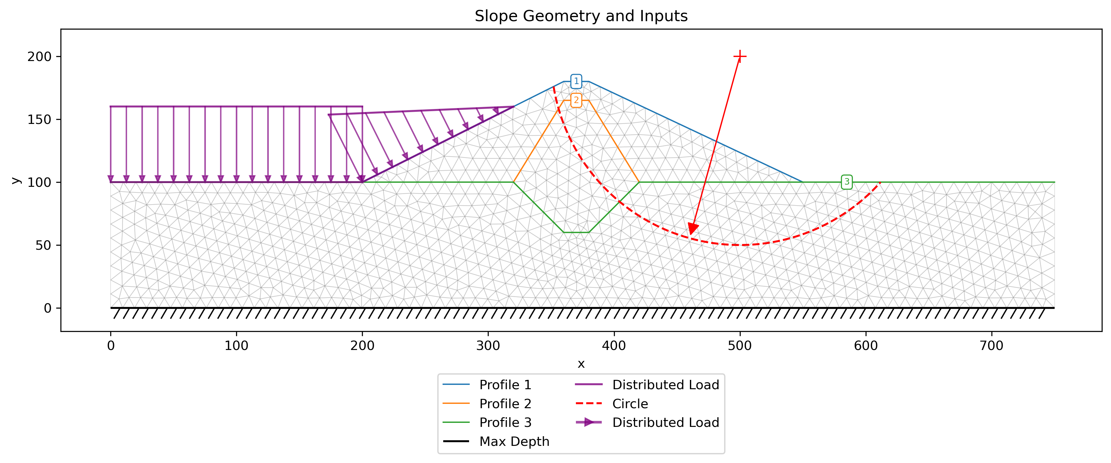
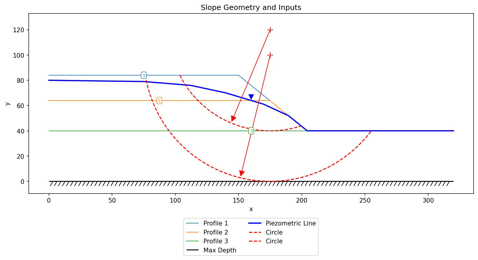
The pore pressures that drive a slope stability analysis can be supplied two ways: from a piezometric line (a hand-drawn phreatic surface, \(u = \gamma_w h_p\)) or interpolated from a finite-element seepage solution. The two are not equivalent — a piezometric line is a simplified estimate of the phreatic surface, while the seepage solution honors the actual flow field and the material permeabilities. The right-facing slope below (a three-layer silt / sand / clay profile from the method-of-slices exercises) is solved both ways on the same single circle (\(X_0 = 175\), \(Y_0 = 100\), tangent to the foundation), so the only thing that changes between the two runs is the pore-pressure model.
Part a — Piezometric line
All three materials use the piezo pore-pressure option, with the phreatic surface entered on the piezo sheet.
Excel input file: xslope_rface_PIEZO_KEY.xlsx
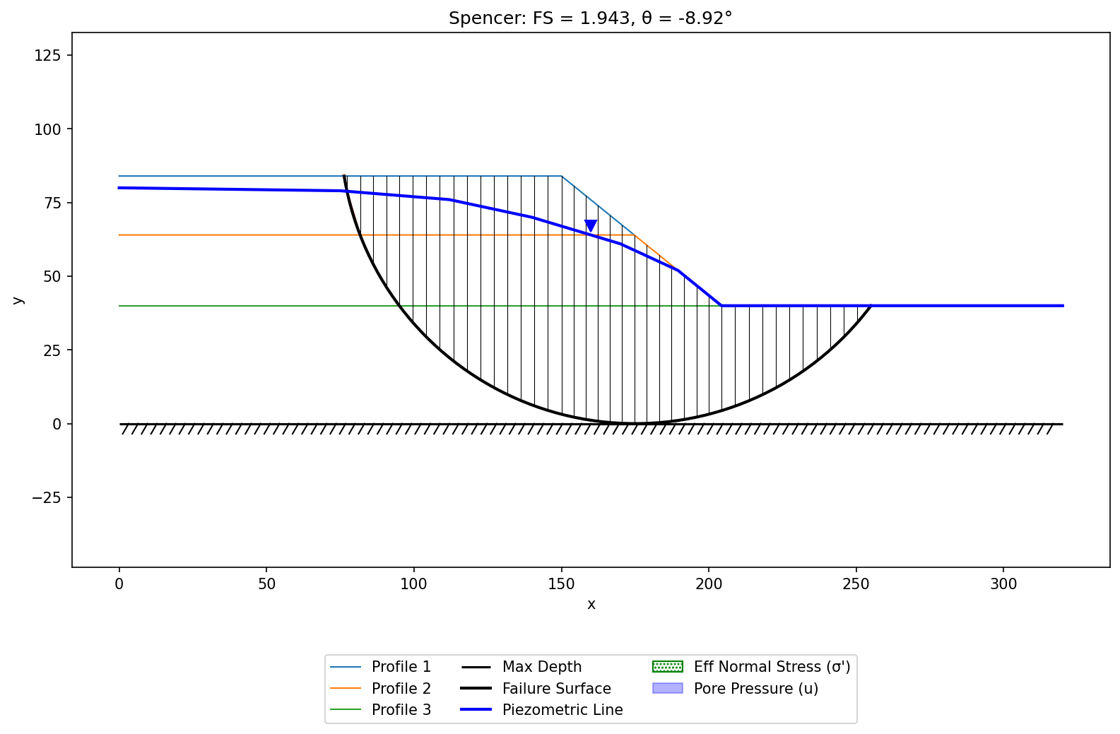
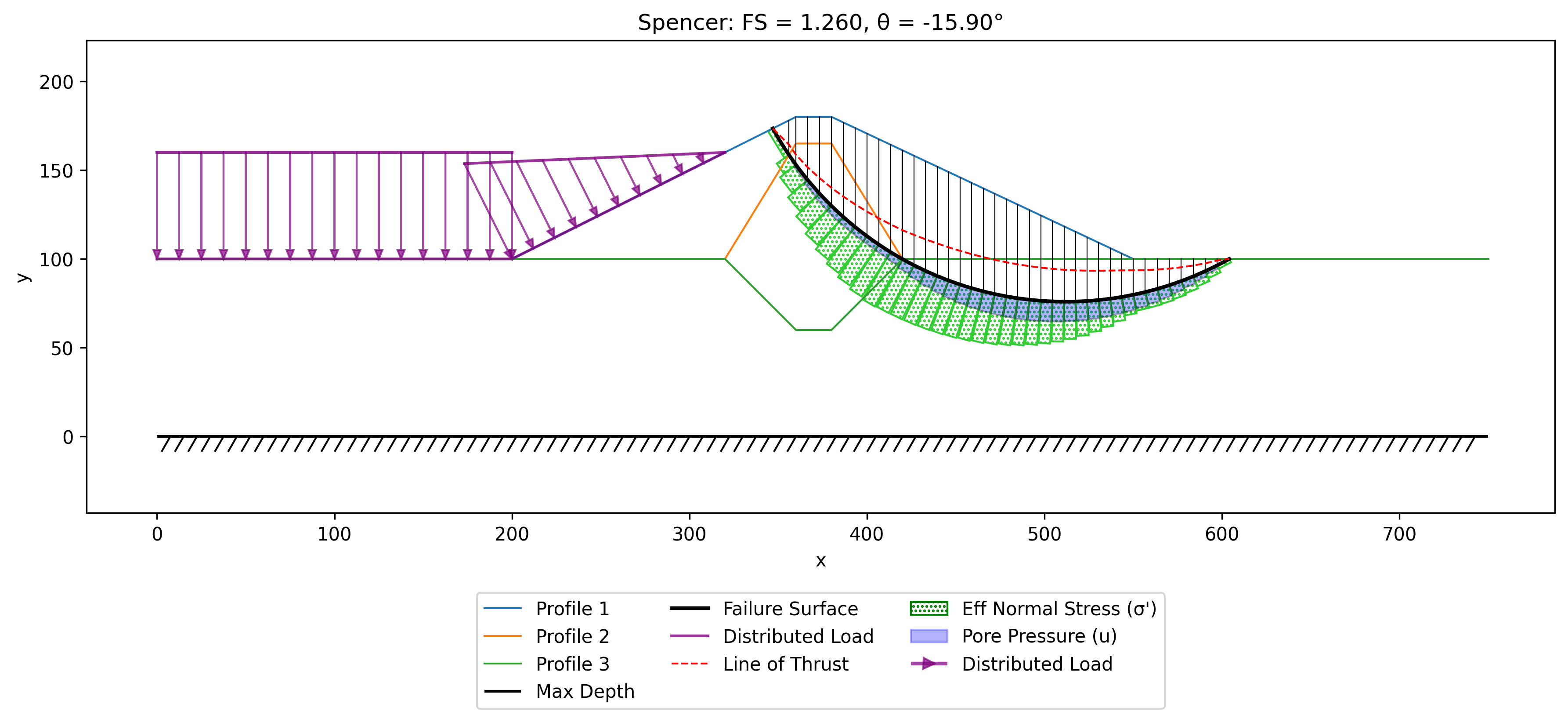
Spencer's method gives FS = 1.94.
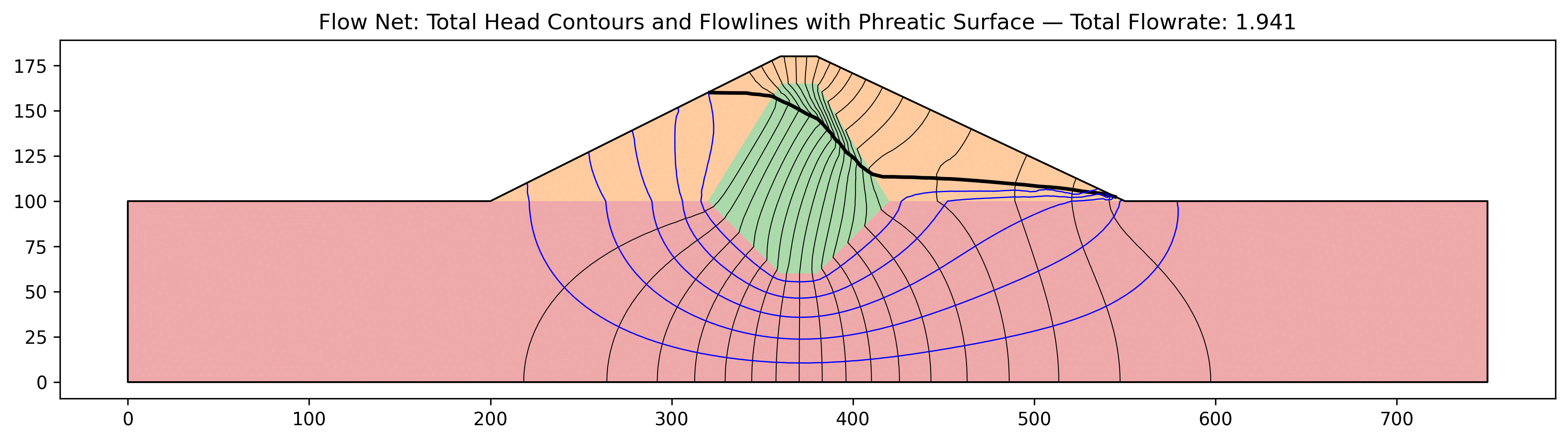
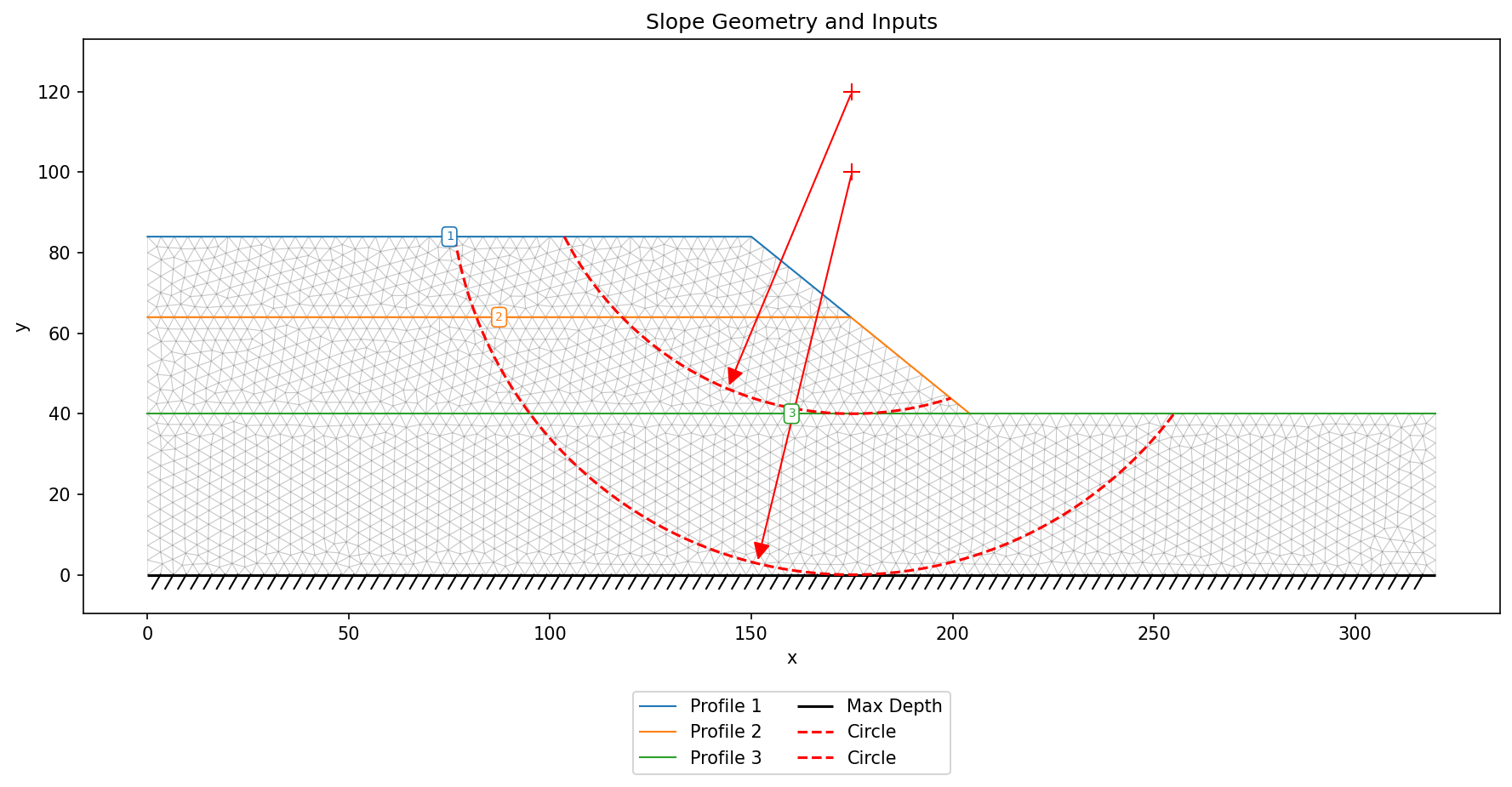
Part b — Seepage-derived pore pressures
The same model is re-run with all three materials switched to the seep option. A finite-element seepage analysis (specified head \(H = 80\) ft upstream, exit face downstream) is run first; its mesh and nodal pore pressures are bundled with the Excel file, imported automatically, and interpolated to each slice base.
Excel input file (mesh and seepage solution bundled alongside): xslope_rface_SEEP_KEY.xlsx
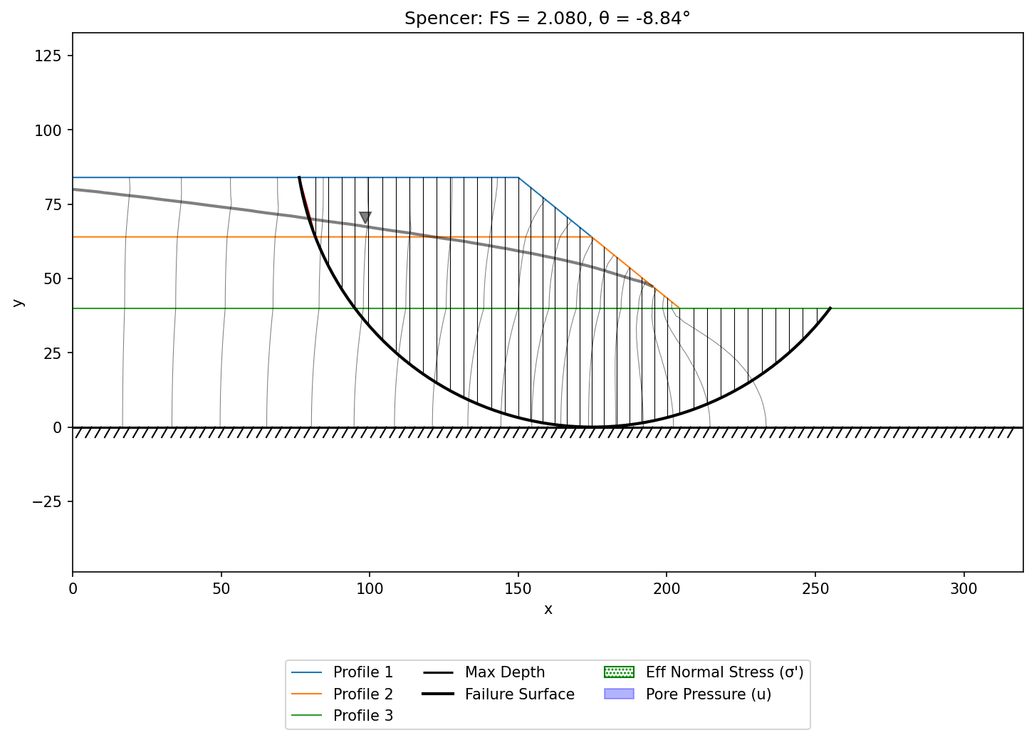
Spencer's method gives FS = 2.08.
Comparison
| Pore-pressure model | OMS | Bishop | Janbu | Corps | Lowe | Spencer | M-P |
|---|---|---|---|---|---|---|---|
| Piezometric line | 1.298 | 1.928 | 1.716 | 2.649 | 2.105 | 1.943 | 1.943 |
| Seepage | 1.473 | 2.068 | 1.863 | 2.798 | 2.258 | 2.080 | 2.081 |
For this slope the piezometric line implies somewhat higher pore pressures than the seepage solution over the body of the slope, so it returns a modestly lower (more conservative) factor of safety — the two agree within about 7%, consistently across all methods. The difference is not always this small, nor always in this direction: where seepage is routed through the more permeable layers and exits along the downstream face, the computed pore pressures near the toe can be far higher than any reasonable piezometric line, dropping the factor of safety dramatically (a near-toe uplift failure). That is exactly why a seepage analysis is preferred whenever seepage is actually occurring.